Canadian Hare Lynx Data

The file hare_lynx.txt contains data on the number of arctic hare and lynx pelts collected by the Hudson’s Bay company in Canada over the course of many years (data obtained from this website).  Do you think the Lotka-Volterra model is an appropriate model to fit to these data?

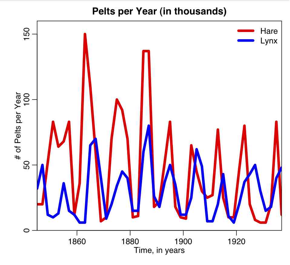
The R script hare_lynx_plot.R plots the Hare Lynx data:

The R script hare_lynx_fit_statistical_model.R uses a statistical model to fit the parameters of the Lotka-Volterra model.  It then uses those parameters to numerically solve the deterministic equations.  The R script produces the plot:

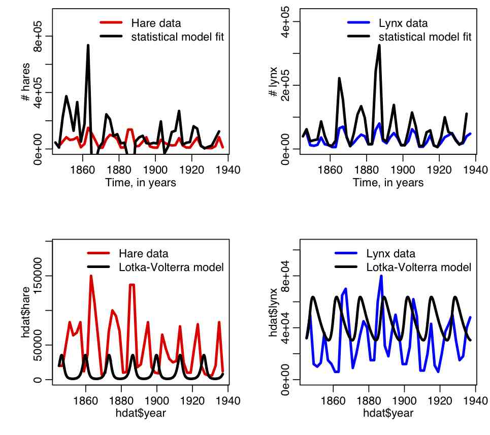
Note that the parameters of the best-fit statistical model result in a very poor fit when employed in numerical solutions of the deterministic ODE’s of the Lotka-Volterra model.  Why do you think this is the case?

Note that when papers discuss “fitting” the Lotka-Volterra model to data like the Hare/Lynx data, they are almost always talking about fitting a statistical model, not fitting the parameters of the deterministic ODE model.

The R script hare_lynx_print_out_data.R prints out the Hare Lynx data set in a format that consists of C++ commands that can be easily copied and pasted into a C++ program.  The files HareLynxData.cpp and HareLynxData.h contain the C++ code for a class that contain vectors filled with the Hare Lynx data set.

Fitting the parameters of the deterministic Lotka-Volterra model to the Hare Lynx data set

There are 6 parameters that we need to fit to the Hare Lynx data set:

1. The initial number of hares
2. The initial number of lynx
3. a
4. b
5. c
6. e

The steps involved in fitting this data set are:

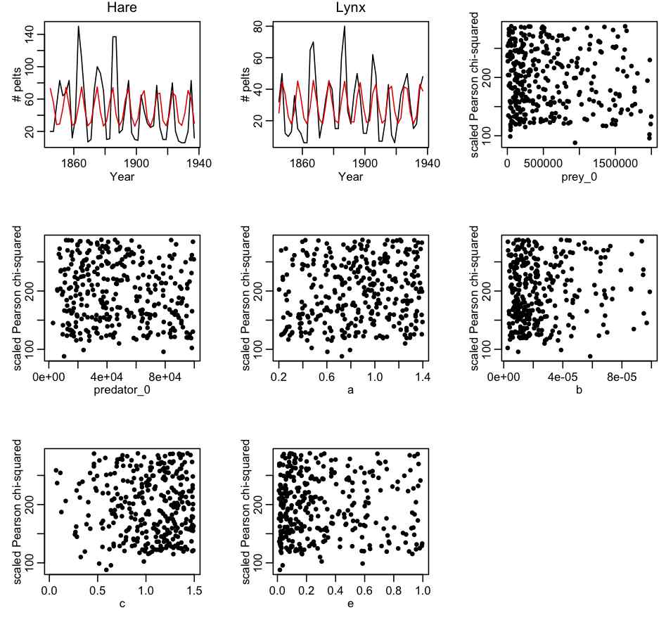
1. Create an R script that uses the deSolve library methods to numerically solve the Lotka-Volterra model.  The R script uniformly samples the 6 parameters over a wide range, and calculates the Pearson chi-squared statistic that compares the data to the model calculated for each set of parameter hypotheses.  Plot the best-fit model over the data.  Re-iterate this step, expanding and contracting the ranges of the parameters to obtain a reasonable fit to the data, and such that the minimum value of the dispersion-corrected chi-squared at each end of the parameter range is at least 16 or so greater than the minimum value.  An example of an R script that implements this process is hare_lynx_fit_step1.R  One run of the R script produces the following plot:
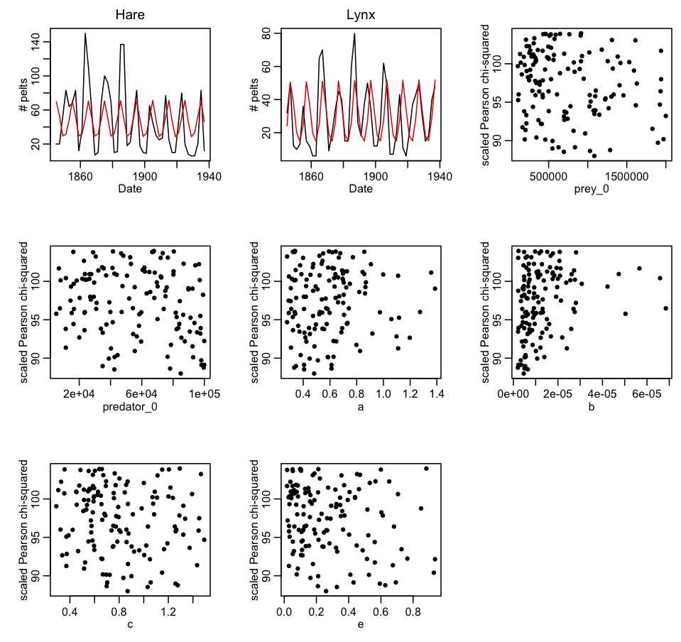
2. Create a C++ program that does the same thing as the R script.  The C++ program will be much more efficient than the R script.  Output the parameter hypotheses and Pearson chi-squared statistics to a file that can be read in by another R script.        Create an R script to read in the output of the C++ program.  Plot the best-fit model over the data, and check that indeed the fit is reasonable.  Correct the Pearson chi-squared statistics for dispersion (if necessary) then plot the corrected Pearson chi-squared statistic vs the hypotheses for each of the parameters in turn.  Ensure that the range of the parameter sampling range is wide enough.  If not, adjust the ranges in the C++ program, and re-iterate step 2.  The first iteration of this process, with 500,000 trials produced the following results (with file hare_lynx_fit_step2.cpp, compiled with makefile makefile_lotka… to run it, type hare_lynx_fit_step2 0 > temp.out):
3. Now that appropriate ranges of the parameters appear to have been identified, use the weighting method described in Module VIII to estimate the best-fit parameters and their covariance matrix and correlation.   Output the results in a format suitable for inclusion in a C++ program. Write a C++ program that randomly samples the parameters from a multivariate Normal distribution using these means and the covariance matrix, and compares the resulting model to the data.  This program is suitable for running in parallel on the Saguaro batch system.