In this past module, we discussed using the Pearson chi-squared statistic to determine the best-fit parameters of an SIR model to influenza B data from the 2007-08 Midwest flu season.   In this module, we will discuss how to find the best-fit parameters using the Negative Binomial likelihood instead.

As discussed in previous modules in this course, the Negative Binomial distribution is an appropriate probability distribution for over-dispersed count data.  The functional form of the distribution takes as its arguments the observed number of counts, Yobs, the predicted number of counts, Ypred (ie; your model prediction, which depends on your model parameters), and a dispersion parameter, ascale.  The dispersion parameter is a measure of the over-dispersion in the data, with ascale~0 indicating that the data are approximately Poisson distributed, and large ascale indicating that the data are very over-dispersed.

While you could just fit over-dispersed count data using a Pearson chi-squared goodness-of-fit statistic applying the McCullagh and Nelder (1989) dispersion correction, this is only really valid when you have sufficient number of counts per bin (say, approximately at least 10 or so) that the stochasticity is approximately Normally distributed rather than Poisson or Negative Binomially distributed.  Thus, for count data that are sparse, Negative Binomial likelihood should always be your statistic of choice for optimizing your model.

But you can use the Negative Binomial likelihood for data for which you could also use dispersion-corrected Pearson chi-squared.  As I mentioned in class, the only time I’ve had the Negative Binomial likelihood method fail on me was when the number of counts in my sample was in the millions… apparently the numerical approximations used to calculate the NB log likelihood are not valid when Yobs or Ypred are extremely large.

The only disadvantage of using the Negative Binomial likelihood for non-sparse count data is readability of your manuscript; the average non-statistician reviewer is generally not familiar with the Negative Binomial likelihood, so you have to be careful in your manuscript to explain in simple terms why you are using this particular statistic as your figure-of-merit in optimizing the parameters of your model.  In general, I tend to keep my analysis methods as simple as possible (without sacrificing robustness or accuracy of my analysis), and describe those methods in plain english, in order to help ensure quick and easy review of my papers.  Our jobs as scientists are not only to do quality research, but to disseminate the results of that research to the outside world in a timely fashion and in easily readable and understandable manuscripts.

As a refresher of what we did in the previous module, here are the results of fitting the SIR model to the Midwest 2007-08 influenza B data using the dispersion-correct Pearson chi-squared statistic (we used the file Flu_example_b.cpp to do the random parameter sampling and calculate the Pearson chi-sq statistic, output to file flu_sim_b.out, and then the results are plotted in R using midwest_flu_b.R):

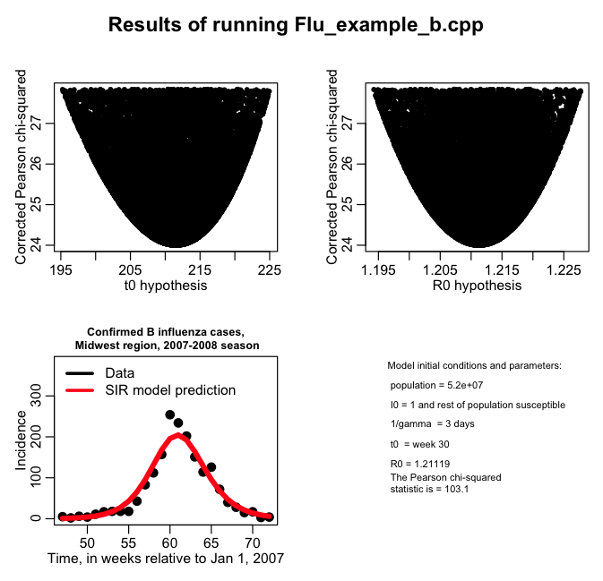
The R script prints out the following 95% CI for t0 and R0:

The central value and 95% CI on R0 is 1.21119 [ 1.19427 , 1.22771 ]
The central value and 95% CI on t0 is 211 [ 195.249 , 224.935 ]

Doing the same thing, but with Negative Binomial Likelihood

For this particular data sample, the dispersion-corrected Pearson chi-squared is probably fine to use as a figure-of-merit statistic, because most of the bins have at least 10 counts in them.  However, it is a nice cross-check to determine if we do indeed get more or less the same central values and confidence intervals if we use the Negative Binomial likelihood instead.

In the file Flu_example_c.cpp I do the parameter sweeps of an SIR model and compare the model estimates to the Midwest flu data and calculate the Negative Binomial likelihood statistic using the NegativeBinomialLikelihood method in the UsefulUtils class.  I also calculate the Pearson chi-squared statistic. You can compile and link the program with the UsefulUtils, FluData, and cpp_deSolve classes using the makefile makefile_flu

Because I am doing a Negative Binomial likelihood fit, in this case I also need to have an extra parameter for the dispersion, which I call adisper.

The parameter hypotheses are randomly sampled in the program from a Normal distribution preferentially sampling about the previous best value (it makes the parameter sampling go quicker).  For each iteration I print out the parameter hypotheses (including adisper), the Negative Binomial negative log likelihood (actually, twice that), and the Pearson chi-squared statistic.

You’ll also note in the program that I control the size of my output file by only printing out results when the parameters are within 5std deviations of the current best-fit hypotheses.  If you don’t do this, you’ll end up with *huge* files when you run on super-computing systems, and most of the lines will contribute nothing to the calculation of the central values and 95% CI on the parameters.

 Submitting the program to run in batch on ASURE

In this past post, we talked about how to submit jobs to the ASU ASURE super-computing system.  Copy the program Flu_example_c.cpp over to the ASURE cluster and compile it using makefile_flu (ensure that you also have the UsefulUtils and cpp_deSolve and FluData class files in the same directory too).  You can use the batch submission script fluc.sh to submit the job in batch.  To submit 10 jobs in batch to run in parallel, type

sbatch --array=1-10 fluc.sh

The output is directed to files of the form flu_c_xxx.out, where xxx is the job number.  To concatenate the files into one, type

cat flu_c*.out >> temp.out

and then you can scp the temp.out file to the file fluc.out on your local machine.

I’ve put the output of the program in fluc.out

The R script midwest_flu_c.R reads in this file and produces the following plot:

and prints out the confidence intervals

The central value and 95% CI on R0 is 1.20737 [ 1.19023 , 1.22274 ]
The central value and 95% CI on t0 is 206 [ 190.128 , 220.046 ]

Compare these confidence intervals to what we got above when we used the dispersion-corrected Pearson chi-squared statistic to do the optimization…. are they close?

Now try plotting the Pearson chi-square statistic and the Negative Binomial negative log likelihood (V9 and V8 in the tdat dataframe, respectively).  What do you see?  How about if you narrow the data frame to only select dispersion coefficients, V5, to be within, say, 0.01 of the minimum value of 0.064?  (note that the Pearson chi-square statistic does not depend on the value of the dispersion coefficient, but the log likelihood of the Negative Binomial statistic does).