
[In this module, we discuss several probability distributions that are important to statistical, mathematical, and computational modeling in the life and social sciences.
Note that the names of probability distributions are proper nouns. Thus, when you write about them, you should always capitalize them.]
Uniform
The Uniform distribution is continuous, defined on x=[a,b].
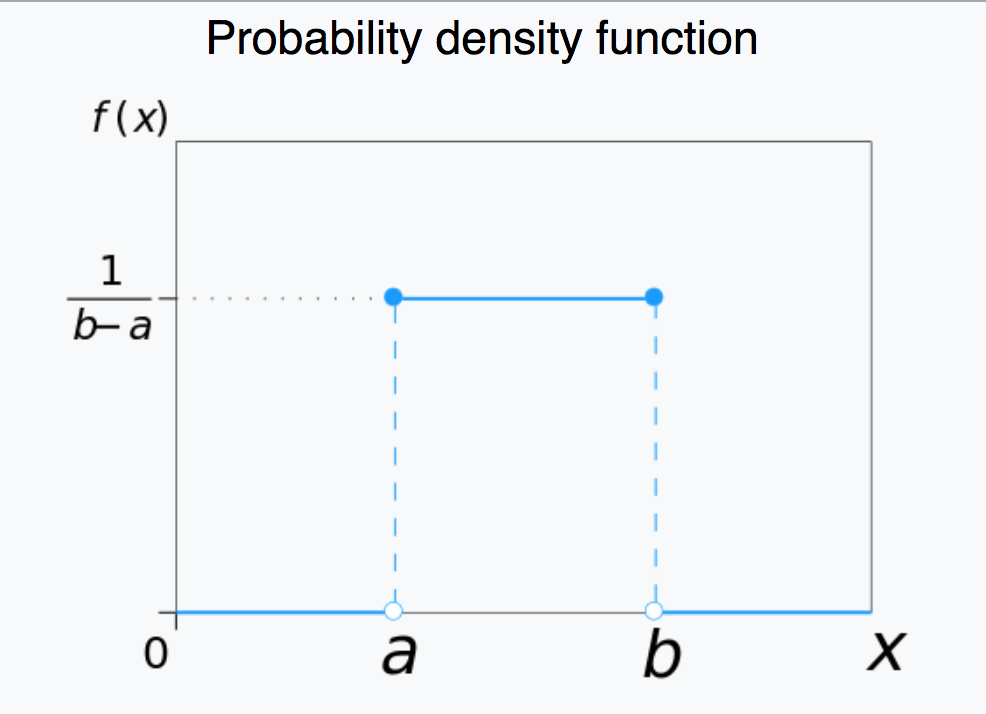
The Uniform probability distribution is key to statistical hypothesis testing. Statistical hypothesis tests assess a p-value, which is the probability of observing the data under the null hypothesis. When the null hypothesis is true, observed p-values will be Uniformly distributed between 0 and 1. If the observed p-value is less than, say, 0.05, we conclude that the null hypothesis is not likely to be true.
The R function runif(N,a,b) generates N random numbers Uniformly distributed between a and b.
The R function punif(x,a,b) yields the integral of the Uniform distribution from a to x. If x<a, it returns 0.
The R function dunif(x,a,b) yields the value of the Uniform probability density at x.
Normal
The Normal distribution is continuous, defined on x=[-inf,+inf]. It has two parameters, the mean, mu, and standard deviation width, sigma.
With the Normal distribution, the probability of observing x, with expected mean mu, and variation sigma^2, is:
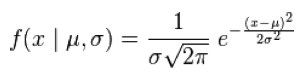
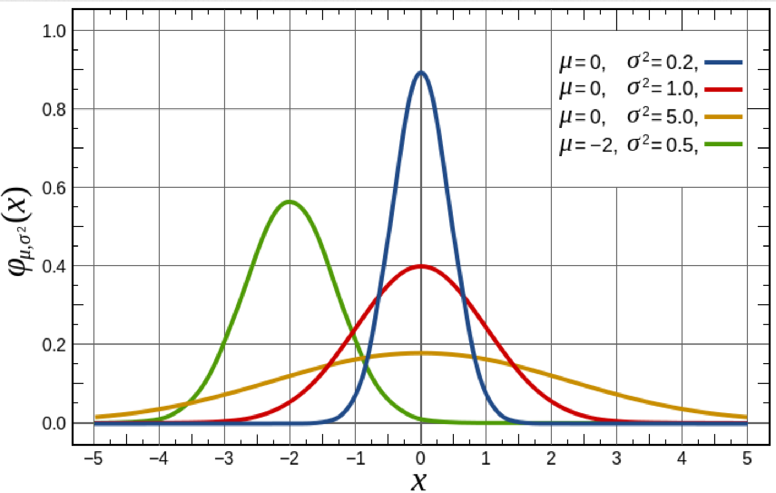
Note that the distribution is symmetric about the mean, and the larger the sigma, the wider the distribution.
The Normal distribution is ubiquitous in applied statistics. A few examples:
- Simple linear regression methods inherently assume that the stochasticity in the data is Normally distributed about some model prediction.
- The Central Limit Theorem says that the mean of random variables drawn from any probability distribution will be approximately Normally distributed.
- The Student’s t-distribution (or simply the t-distribution) is a continuous probability distribution that arises when estimating the mean of a Normally distributed population in situations where the sample size is small and population standard deviation is unknown.
Unless you are told otherwise in a manuscript, assume uncertainties on estimates in papers are Normally distributed; thus if the paper says (for instance) that the infectious period of a disease has an average of 3 days with standard deviation 1, you should assume that what they mean is that the posterior probability distribution they obtain for the infectious period is Normally distributed with mu=3 and sigma=1.
As we will see below, many probability distributions approach the Normal distribution under certain conditions.
The R function rnorm(N,mu,sigma) generates N random numbers Normally distributed with mean mu and std deviation sigma.
The R function pnorm(x,mu,sigma) yields the integral of the Normal distribution from -inf to x. If you set the optional argument lower.tail=F, then pnorm(x,mu,sigma,lower.tail=F) yields the integral of the Normal distribution from x to +inf, which is the same as 1-pnorm(x,mu,sigma).
If X are a set of numbers randomly drawn from the Normal distribution with mean mu and sigma, then pnorm(X,mu,sigma) will be Uniformly distributed between 0 and 1.
If you don’t know the true underlying mu and sigma, and histogram pnorm(X,mu,sigma), if the hypothesized mu is too low/high, the histogram will pile up at 1/0. If the hypothesized sigma is too low, the histogram will pile up at 0 and 1. If the hypothesized sigma is too high, the histogram will pile up in the middle. It is only when the hypothesized mu and sigma are very close to the true values that underlie the random X that the distribution of pnorm(X,mu,sigma) approaches the Uniform distribution.
It is important to note that if x is a random number drawn from Normal(mu,sigma), then pnorm(x,mu,sigma) will be a Uniformly distributed random number between 0 and 1. Thus, approximately 5% of the time, pnorm(x,mu,sigma) will yield a number less than 0.05.
The R function dnorm(x,mu,sigma) yields the value of the Normal PDF at x.
The R function qnorm(z,mu,sigma) for 0<=z<=1 returns the value of x such that the integral of the Normal distribution from 0 to x is equal to z.
Poisson
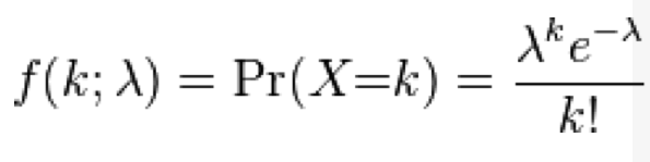
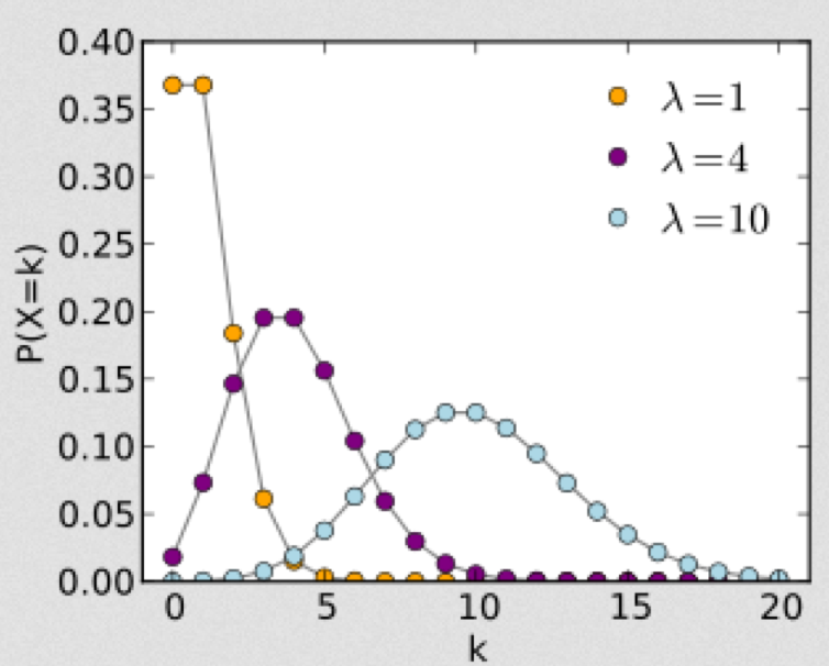
The Poisson distribution is discrete, defined in integers x=[0,inf]. It has one parameter, the mean lambda.
With the Poisson distribution, the probability of observing k events when lambda are expected is:
Poisson stochasticity can underlie count data. It has been used, for instance, to describe the stochastic variation in animal litter sizes, and household sizes (once zero truncated).
As the parameter lambda gets large (say, greater than 10 to 25 or so), the Poisson distribution approaches the Normal distribution with mu=lambda, and sigma=sqrt(lambda). When you hear me say that “the stochasticity in count data is not in the Normal regime”, that’s my shorthand way of saying that the data points are all less than 25 or so. It is convenient that if the counts in the data set are all more than 25 or so, we can often use methods like standard linear regression that assume that the stochasticity is Normal (after accounting for things like heteroscedasticity that is, but that’s beyond the scope of this current discussion).
The R function rpois(N,lambda) generates N random numbers Poisson distributed with mean lambda.
The R function ppois(x,lambda) yields the sum of the Poisson probability density from 0 to x. If you set the optional argument lower.tail=F, then ppois(x,lambda,lower.tail=F) yields the sum of the Poisson distribution from x+1 to inf.
If X are a set of numbers randomly drawn from the Poisson distribution with mean lambda, then ppois(X,lambda) will be approximately Uniformly distributed between 0 and 1 if lambda is large enough that the distribution is in the Normal regime.
For large lambda, if x is randomly drawn from Pois(lambda), then ppois(x,lambda) will approach a Uniformly distributed random number between 0 and 1. For small lambda, ppois(x,lambda) has a discrete nature inconsistent with the Uniform probability distribution.
The R function dpois(x,lambda) yields the value of the Poisson probability density at x.
Binomial
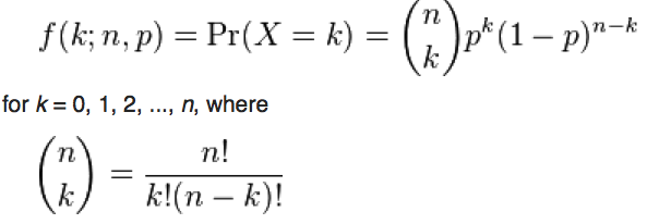
The Binomial distribution is a discrete probability distribution, describing the number of x successes out of n trials when probability of success per trial is p. It is defined on integers x=[0,n]
With the Binomial distribution, the probability of k successes out of n trials, when the probability of success is k, is:
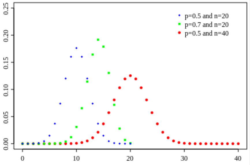
When both n*p and n*(1-p) are greater than around 25, (or n>9*p/(1-p) and n>9*p/(1-p)) the Binomial distribution for k approaches the Normal distribution with mu=np, and sigma=sqrt(np(1-p)).
The Binomial distribution of k also approaches the Poisson distribution under some circumstances; if n>20 and p<0.05, then the distribution of k approaches the Poisson distribution with lambda=np.
The R function rbinom(N,n,p) generates N random numbers Binomially distributed with n trials with a probability of success equal to p.
The R function pbinom(x,n,p) yields the sum of the Binomial distribution from 0 to x. If you set the optional argument lower.tail=F, then pbinom(x,n,p,lower.tail=F) yields the sum of the Binomial distribution from x+1 to n.
When X are random numbers drawn from the Binomial distribution with parameters such that it approaches the Normal distribution, then the distribution of pbinom(X,n,p) will be approximately Uniformly distributed between 0 and 1.
The R function dbinom(x,n,p) yields the value of the Binomial probability density at x.
Another useful R function related to the Binomial distribution is binom.test(k,n,p). It calculates the estimated value of p from k/n, and also returns the 95% CI on that estimate (ie; 95% of the time, the true value of p that underlies the data will lie within the estimated confidence interval). It also assesses the probability that you could observe k successes out of n trials if the probability of success is truly p. A good example of the utility of this method is an analysis I did recently, debunking the idea that sunspot activity causes influenza pandemics.
Exponential
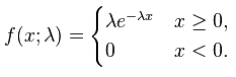
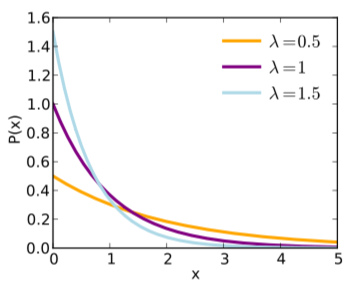
The Exponential probability distribution is continuous, defined on t=[0,inf], with one parameter, lambda. The mean of the distribution is 1/lambda, and the standard deviation is 1/lambda. It is often used to as the probability distribution underlying the wait time between events.
With the exponential distribution, the probability of observing a wait time between events, x, when the expected average wait time is 1/lambda is:
The Exponential distribution with parameter lambda is intimately related to the Poisson distribution with parameter lambda; the Poisson distribution describes the number of events observed in one unit of time when the waiting time between events is Exponentially distributed.
The Exponential distribution also describes the time between events in a Poisson process. For instance, assume that lambda babies are on average born in a hospital each day, with underlying stochasticity described by the Poisson distribution. The probability distribution for the wait time (in days) between babies is lambda*exp(-t*lambda)
The Exponential distribution inherently underlies the probability distribution for state soujourn times in compartmental models of biological processes and disease, like the SIR model. Interestingly, the exponential probability distribution is “memory-less”; for example, for an SIR model, this means that the probability of an individual leaving the infectious state between times t and t+Δt (given that they are in the infectious state at time T) does not depend on t… it only depends on Δt! For things like agent based modeling, this property is really convenient, because it means you don’t have to keep track of how long someone has been infectious in order to determine their probability of recovering in a time step.
Unfortunately, assuming that state sojourn times are exponentially distribute in things like a disease model really isn’t very realistic. After all, it implies that the most probable time to recover is at time zero after being infected, or the most probable time to die is immediately after being born! Rather, there is usually a very low probability of recovering immediately after infection, or dying immediately after being born. As an example, here is the distribution of time to death after first showing symptoms of victims in the 1919 influenza pandemic in Sydney Australia. It is rather obviously not Exponentially distributed! In the next section we’ll describe a probability distribution that does a better job of describing these kinds of observations.

The R function rexp(N,lambda) generates N random numbers Exponentially distributed with mean 1/lambda.
The R function pexp(x,mu,lambda) yields the integral of the Exponential probability density from 0 to x.
The R function dexp(x,lambda) yields the value of the Exponential probability density at x.
Gamma
A much better probability distribution for sojourn times in compartmental biological and epidemiological models is the Gamma distribution. It is a continuous, defined on t=[0,inf], and has two parameters called the scale factor, theta, and the shape factor, k.
When the shape parameter is an integer, the distribution is often referred to as the Erlang distribution.
The PDF of the Gamma distribution is
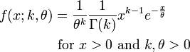
For various values of k and theta the probability distribution looks like this:

Notice that when k=1, the Gamma distribution is the same as the Exponential distribution with lambda=1/theta. The mean of the distribution is mu=k*theta, and the variance is sigma^2=k*theta^2.
When k>1, the most probable value of time (“x” in the function above) is no longer 0. This is what makes the Gamma distribution much more appropriate to describe the probability distribution for time spent in a disease state.
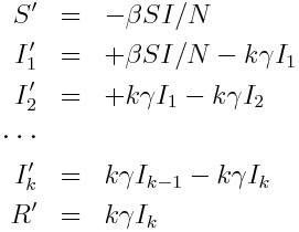
The Erlang distribution is the distribution of the sum of k independent Exponentially distributed random variables with mean theta. It turns out that this property provides a convenient means to incorporate an Erlang distributed probability distribution for the sojourn time into a compartmental model in a straightforward fashion; for instance, assume that the sojourn time in the infectious stage of an SIR model is Erlang distributed with k=2 and theta = 1.5 (with 1/gamma = k*theta)… simply make k infectious compartments, each of which (but the last) flows into the next with rate gamma*k. The last compartment flows into the recovered compartment:
Note that the Gamma distribution is not memoryless; the probability of leaving a state between times t and t+Δt depends on how long the individual has been in the state. To include realistic Gamma distributed state sojourn times in an agent based model, there is thus increased computational overhead involved in keeping track of how long each individual has been in their particular state.
The R function rgamma(N,scale,shape) generates N Gamma distributed random numbers (the scale factor is theta, and the shape factor is k in the above equation for the PDF).
The R function pgamma(x,scale,shape) yields the integral of the Gamma distribution from 0 to x.
The R function dgamma(x,scale,shape) yields the value of the Gamma probability density at x.
Beta
The Beta distribution is continuous, and defined on x=[0,1]
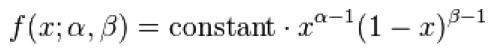
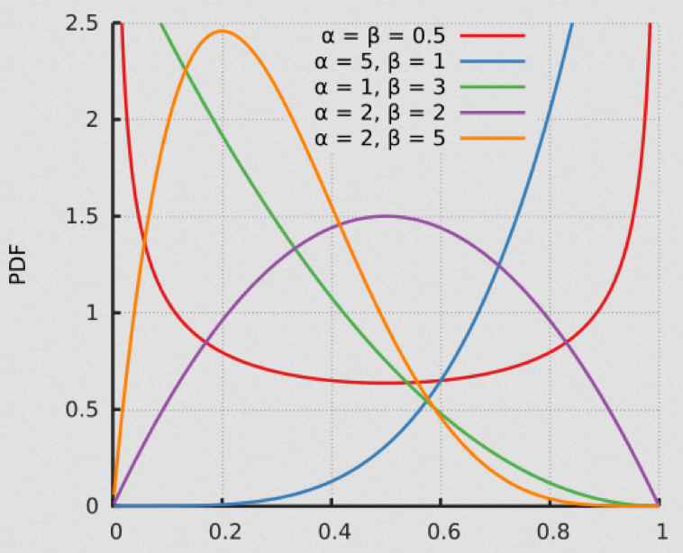
This is a rather specialized distribution with somewhat limited applicability in modeling in the life and social sciences, but I include it here because it is quite useful when including things like economic or other disparities in a model.
Negative Binomial
The Negative Binomial distribution, like the Poisson distribution, is a discrete probability distribution defined for integers from 0 to infinity. Thus, it is an example of a probability distribution that underlies stochasticity in count data.
The Wikipedia pages describing the many various probability distributions are generally excellent. However, the Negative Binomial distribution is one of the few distributions that (for application to epidemic/biological system modelling), I do not recommend reading the associated Wikipedia page. Instead, one of the best sources of information on the applicability of this distribution to modeling in the life and social sciences is this PLoS paper on the subject: Maximum Likelihood Estimation of the Negative Binomial Dispersion Parameter for Highly Overdispersed Data, with Applications to Infectious Diseases As the paper discusses, the Negative Binomial distribution is the distribution that underlies the stochasticity in over-dispersed count data. Over-dispersed count data means that the data have a greater degree of stochasticity than what one would expect from the Poisson distribution… they appear to have greater random variation.
Recall that for count data with underlying stochasticity described by the Poisson distribution that the mean is mu=lambda, and the variance is sigma^2=lambda. In the case of the Negative Binomial distribution, the mean and variance are expressed in terms of two parameters, mu and alpha (note that in the PLoS paper above, m=mu, and k=1/alpha); the mean of the Negative Binomial distribution is mu=mu, and the variance is sigma^2=mu+alpha*mu^2. Notice that when alpha>0, the variance of the Negative Binomial distribution is always greater than the variance of the Poisson distribution.
There are several other formulations of the Negative Binomial distribution, but this is the one I’ve always seen used so far in analyses of biological and epidemic count data.
The PDF of the Negative binomial distribution is (with m=mu and k=1/alpha):
In the file negbinom.R, I give a function that calculates the PDF of the Negative Binomial distribution, and another function that produces random numbers drawn from the Negative Binomial distribution. Don’t use the built-in R functions as they are for the Negative Binomial distribution, because the parameters are not expressed in the form of the PDF above.
To run the script, the R library sfsmisc must be installed. If it is not already installed, type
install.packages("sfsmisc")
then choose a download site located near you. Then, in the R command line, type
source("negbinom.R")
The script produces the following plot:
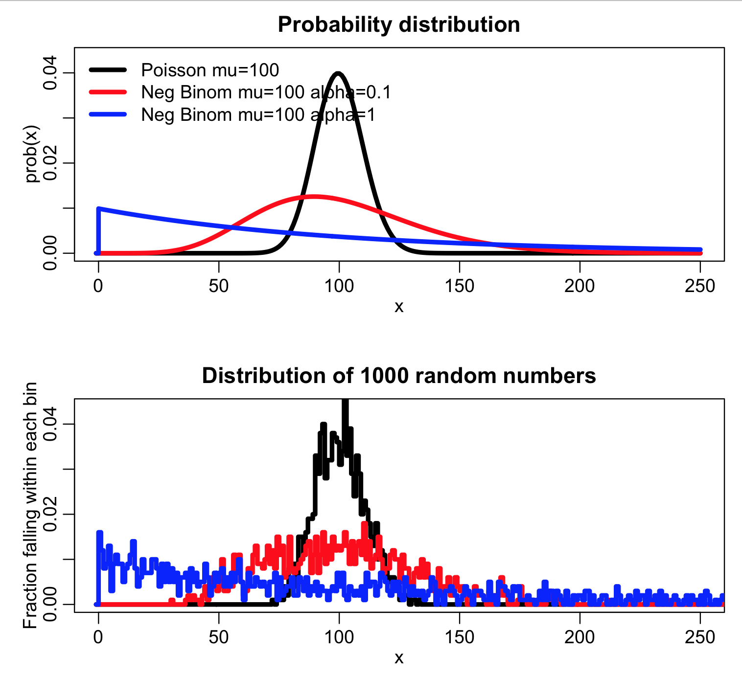
The script also histograms ppois(X,lambda) for the random numbers X randomly drawn from the three probability distributions. Recall that for random numbers drawn from the Poisson probability distribution with large lambda (such that the distribution is in the Normal regime) ppois(X,lambda) should be approximately Uniformly distributed between 0 and 1:
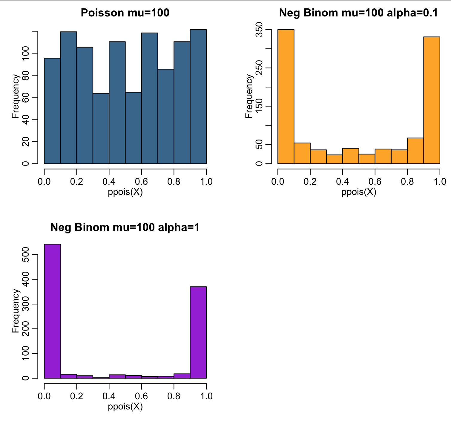
Notice that for the over-dispersed simulated data, ppois(X,lambda) piles up at 0 and 1. This is a nice visual test to determine whether or not data that you think is Poisson distributed is in fact over dispersed.