[In this module, students will become familiar with a formalism for structuring information related to compartmental models. This formalism is very helpful when developing either Markov Chain Monte Carlo or Stochastic Differential Equations for stochastic simulation of the model]

A good, but much more mathematical, introduction to the material discussed here can be found in the paper Construction of Equivalent Stochastic Differential Equation Models by Allen et al (2008).

• Step 1: write down the model equations, and count the number of compartments, K
• Step 2: write down all possible changes of +/-1 individual in the compartments that can occur, and then count the number of possible changes, J
• Step 3: write down the possible changes as a JxK matrix, lambda
• Step 4: determine the average number of times that each of the J transitions will take place in time delta_t
• Step 5: make a summary table
• Simple example: predator prey model
• More complicated example: SIRS model with vital dynamics

Step 1: write down the model equations, and count the number of compartments, K

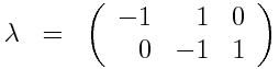
Say we have a compartmental model for some dynamical system, with k=1,2,…,K compartments.  In the case of an SIR model, we have three compartments; the susceptible (S), infected (I), and recovered (R).  The set of ordinary differential equations describing the model is:

The first step in this formalism is to write down the set of equations describing your dynamical system.  Then count the number of compartments in your system, K.

Step 2: write down all possible changes of +/-1 individual in the compartments that can occur, and then count the number of possible changes, J

Because each compartment contains individuals, the smallest change that can occur to any one compartment is plus or minus one individual. The next step in the formalism is to write down all possible changes of +/-1 individuals that can occur in the compartments.  For the SIR model we have

1. S can change by -1, and I changes by +1 (infection)
2. I can change by -1, and R changes by +1 (recovery)

For this particular model, the number of possible changes is J=2.

Step 3: write down the possible changes as a JxK matrix, lambda

The next step in the formalism is to write down the possible +/-1 changes as a JxK matrix, that we will call lambda.  Note that in the first set of changes above, delta_S=-1, delta_I=+1, and delta_R=0, and in the second set of equations delta_S=0, delta_I=-1, and delta_R=+1.  Thus, we get for lambda

Step 4: determine the number of times that each of the J changes will take place in time delta_t

In a past module, we talked about how to determine the time step needed to ensure that on average just one change occurs in a compartmental model; essentially, it amounts to summing up the flow between compartments (plus adding in the flow of births and/or deaths, if they occur in the model).  For the SIR model, the time step needed to ensure just one change on average is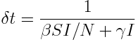
  Eqn 1.

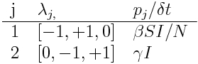
The number of times that a particular change occurs in time delta_t is the rate of flow associated with that change, times delta_t. Thus, to determine those numbers, the next step is to write down the rate of flow that is associated with each of the J possible changes in your compartments.  This rate of flow, times delta_t, is the average number of times, p_j, that there will be change j during delta_t.  When delta_t is defined as in Eqn 1, these numbers sum to one. Thus, for the example of the SIR model, we have

1. delta_S =-1, and delta_I =+1 (p_1=delta_t*beta*S*I/N)
2. delta_I=-1, and delta_R=+1 (p_2=delta_t*gamma*I)

Thus, when delta_t is defined as in Eqn 1, the p_j form a vector of length J that sums to one.

Step 5: make a summary table

A nice way to express all of the above is to make a summary table, like this:

Easy! 

Simple example: predator prey model

(image source)

The equations for a simple predator (y) prey (x) model are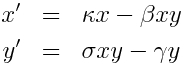

We assume in this simple model that the only way the prey can die is if it is eaten by a predator. The model has K=2 compartments. There are J=4 different changes that can result in a change in the compartments of +/-1 individual.  An x can either be born with rate kappa*x, or die with rate beta*x*y, and a y can either be born with rate sigma*x*y, or die with rate gamma*y.  We get the summary table for this model is thus:

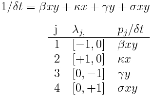
Note that there are no flows between the K=2 compartments in this model, however there are interaction terms between the compartments. We’ll in a see later module, when we discuss SDE’s in further detail, that models with no flow between compartments simplify things in a nice way.

More complicated example: SIRS model with vital dynamics

In this case, we modify our simple SIR model to include births and deaths with rate mu, and a return back to the S compartment from the R compartment with rate alpha.  The model equations are: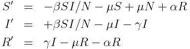

We thus have K=3 compartments.  Unlike the predator prey model, here we have flows between the compartments.

(image source)

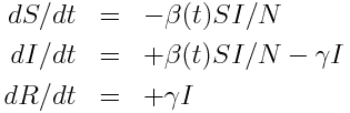
There are J=7 changes that can result in a change of +/-1 to the compartments.  They are

1. delta_S=-1, delta_I=1 (infection, rate beta*S*I/N)
2. delta_S=1, delta_R=-1 (re-susceptibility, rate alpha*R)
3. delta_I=-1, delta_R=+1 (recovery, rate gamma*I)
4. delta_S=-1 (death of S, rate mu*S)
5. delta_I=-1 (death of I, rate mu*I)
6. delta_R=-1 (death of R, rate mu*R)
7. delta_S = +1 (birth of a new susceptible, rate mu*N)

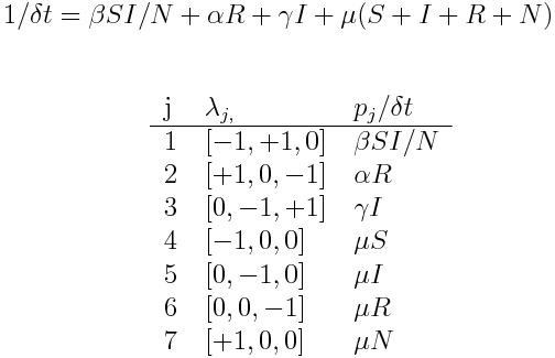
We thus get delta_t and the summary table are: