In this module we will discuss how to conduct one-sample and two-sample Students t-tests of sample means when the variance of the sample is unknown, testing the equality of the means of several samples, and z-test of sample means when the variance is known.

Contents:

• Students t-test of the mean of one sample
• Example of Students t-test of the mean of one sample
• Students t-test comparing the means of two samples
• Example of Students t-test comparing the means of two samples
• Limitations of the Students t-test
• Testing for equality of more than two means (ANOVA)
• One and two sample Z-tests

The Student t distribution arises when estimating the mean of a Normally distributed population, particularly when sample sizes are small, and the true population standard deviation is unknown.

Using the Students t-test to test whether a sample mean is consistent with some value

If we wish to test the null hypothesis that the mean of a sample of Normally distributed values is equal to mu, we use the Students t statistic

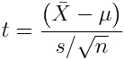
with degrees of freedom

where s is the sample standard deviation, and n is the sample size. The R t.test(x,mu) method tests the null hypothesis that the sample mean of a vector of data points, x, is equal to mu under the assumption that the data are Normally distributed.

Note that it is up to the analyst to ensure that the data are, in fact Normally distributed. The shapiro.test(x) method in R employs the Shapiro-Wilk test to test the Normality of the data.

Example of one sample t-test

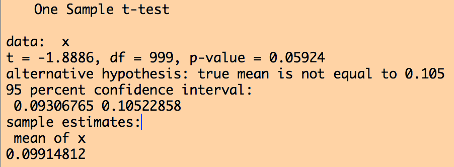
The following R code shows an example of using the R t.test() method to do a one sample t test:

set.seed(832723)
n_1 = 1000
s = 0.1
mean_1 = 0.1
x = rnorm(n_1,mean_1,s)
t.test(x,mu=0.105)

which produces the output:

Testing whether or not means of two samples are consistent with being equal

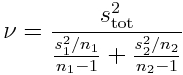
The independent two sample t-test tests whether or not the means of two samples, X1, and X2, of Normally distributed data appear to be drawn from distributions with the same mean. If we assume that the two samples have unequal variances, the test statistic is calculated as

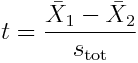
with, under the assumption that the variances of the two samples are unequal

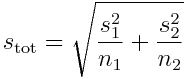
with s_1^2 and s_2^ being the variances of the individual samples.

The t-distribution of the test will have degrees of freedom

This test is also know as Welch’s t-test.

If we instead assume that the two samples have equal variances, then we have

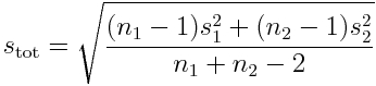
and the test has degrees of freedom

The R method t.test(x,y) tests the null hypothesis that two Normally distributed samples have equal means.  The option var.equal=T implements the t-test under the hypothesis that the sample variances are equal.

When using the var.equal=T option, it is up to the analyst to do tests to determine whether or not the variances of the two samples are in fact statistically consistent with being equal.  This can be achieved with the var.test(x,y) method in R, which compares the within sample variances to the variance of the combination of the x and y samples.

Example of two sample t-test

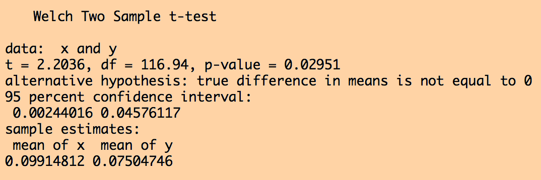
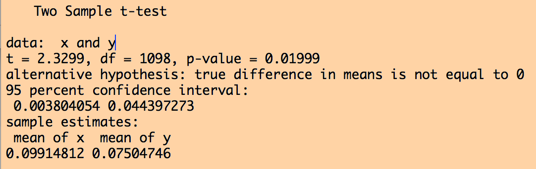
The following example code shows an implementation of the two sample t-test, first with the assumption with unequal variances, then with the assumption of equal variances (which is not true for this simulated data):

set.seed(832723)

n_1 = 1000
n_2 = 100
s_1 = 0.1
s_2 = 0.11
mean_1 = 0.1
mean_2 = 0.08
x = rnorm(n_1,mean_1,s_1)
y = rnorm(n_2,mean_2,s_2)

print(t.test(x,y))
print(t.test(x,y,var.equal=T))

which produces the following output:

Limitations of Students t-test

Limitations of using Students-t distribution for hypothesis testing of means: hypothesis testing of sample means with the Student’s-t distribution assumes that the data are Normally distributed. In reality, with real data this is often violated. When using some statistic (like the Students-t statistic) that assumes some underlying probability distribution (in this case, Normally distributed data), it is incumbent upon the analyst to ensure that the data are reasonably consistent with that underlying distribution; the problem is that the Students-t test is usually applied with very small sample sizes, in which case it is extremely difficult to test the assumption of Normality of the data. Also, we can test the consistency of equality of at most two means; the Students-t test does not lend itself to comparison of more than two samples.

Comparing the means of more than two samples, under the assumption of equal variance 

Under the assumption that several samples have equal variance, and are Normally distributed, but with potentially different means, one way to test if the sample means are significantly different is to chain the samples together, and create a vector of factor levels that identify which sample each data point represents.

The R aov() method assesses the ratio of average of the within group variance to the total variance, using the F statistic:

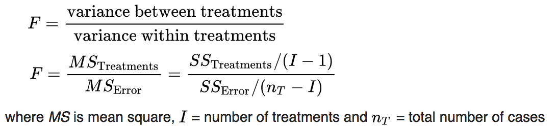
This is known as an Analysis of Variance (ANOVA) analysis.  Essentially, the F-test p-value of tests the null hypothesis that the variance of the residuals of model is equal to the variance of the sample.

Example:

set.seed(832723)
n_1 = 1000
n_2 = 100
n_3 = 250
s = 0.1
mean_1 = 0.1
mean_2 = 0.12
mean_3 = 0.07
x = rnorm(n_1,mean_1,s)
y = rnorm(n_2,mean_2,s)
z = rnorm(n_3,mean_3,s)
vsample = c(x,y,z)
vfactor = c(rep(1,n_1)
           ,rep(2,n_2)
           ,rep(3,n_3))
a = aov(vsample~factor(vfactor))
print(summary(a))

which produces the output:

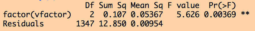
But the thing I don’t like about the aov() method is that it doesn’t give quantitative information about the means of the sample for the different factor levels.  Thus, an equivalent technique that I prefer is to use the R lm() method and regress the sample on the factor levels

myfit = lm(vsample~factor(vfactor))
print(summary(myfit))

which produces the output:

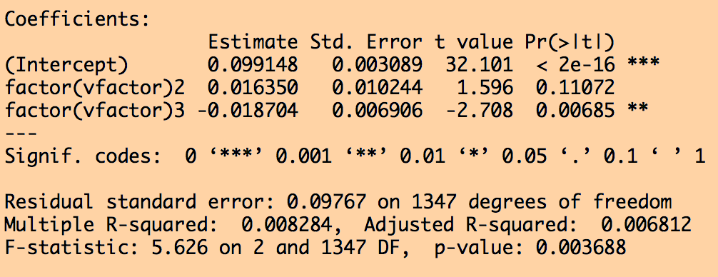
Now we have some information on how the means of the factor level differ. Note that the F statistic p-values from the lm() and aov() methods are the same.

Z test of sample mean

If you know what the true population std deviation of the data are, sigma, and want to test if the mean of the sample is statistically consistent with some value, you can use the Z-test

For a given cut on the p-value, alpha, with a two sided Z-test, we reject the null hypothesis when the absolute value of |bar(X)-mu| is greater than Z_(alpha/2), where Z_(alpha/2) is the (100-alpha/2) percentile of the standard Normal distribution.

You can also do one-sided Z-tests where you test the significance of Z<mu or Z>mu.  However, unless you have very good reason to assume some direction to the relationship, always do a two-sided test of significance instead.

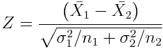
For the two sample Z test, to compare the means of two samples when the variance is known for both, we use the statistic

Now, recall that for large n, the Students t distribution approaches the Normal:

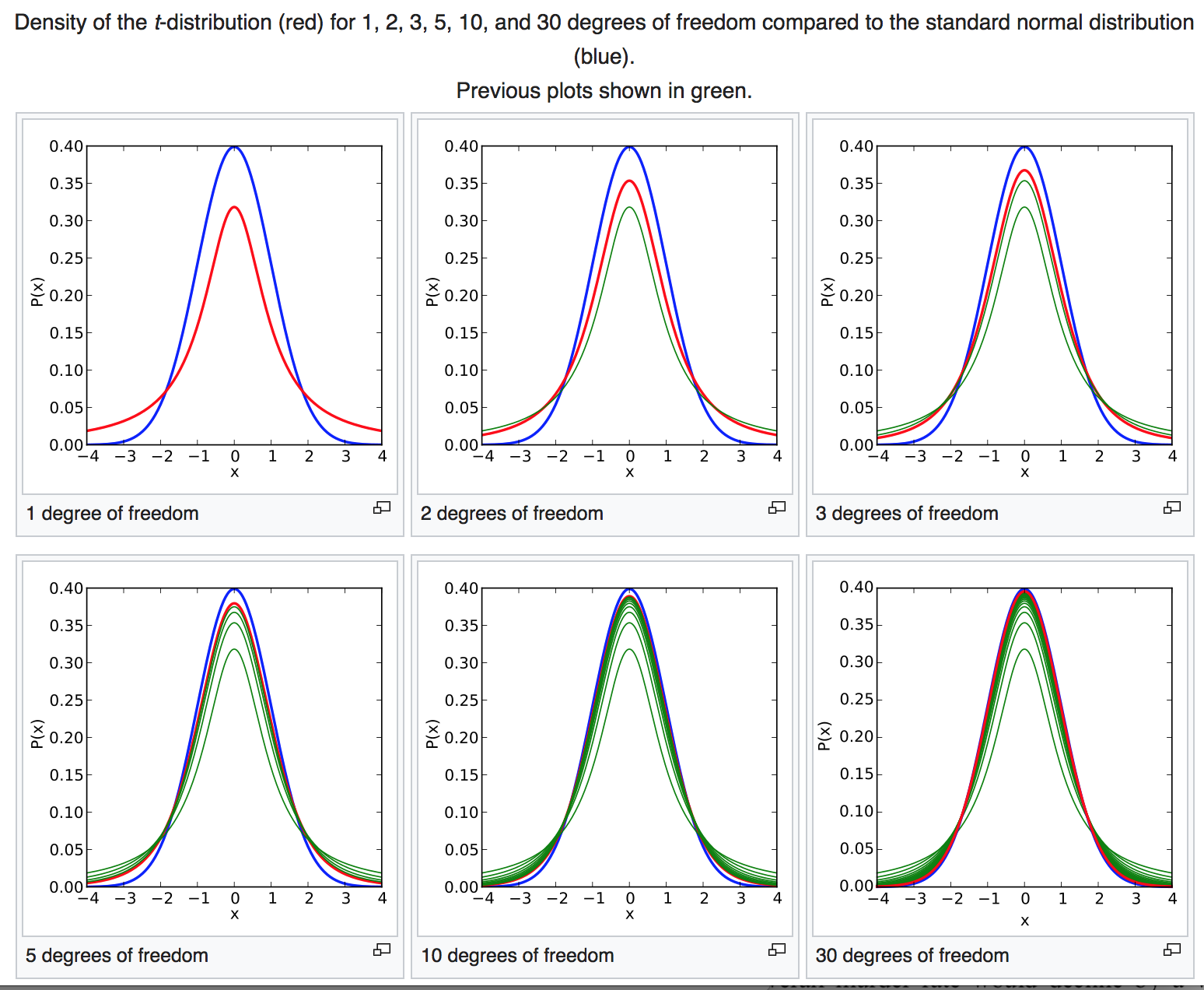
For this reason, when the sample size is large, you can equivalently do a Z-test instead of a t-test, estimating sigma from the std deviation width of the sample.

The BSDA library in R has a z.test() function that either performs a one sample Z test with z.test(x,mu,sigma.x) or a two sample Z test comparing the means of two samples with z.test(x,y,sigma.x,sigma.y)

Example of one and two sample Z-tests compared to Student t-tests

To run the following code, you will need to have installed the BSDA library in R, using the command install.packages(“BSDA”), then choosing a download site relatively close to your location.

First let’s compare the Z-test and Students t-test for fairly large sample sizes (they should return p-values that are quite close):

require("BSDA")
set.seed(832723)
n_1 = 1000
n_2 = 100
s_1 = 0.1
s_2 = 0.11
mean_1 = 0.1
mean_2 = 0.08
x = rnorm(n_1,mean_1,s_1)
y = rnorm(n_2,mean_2,s_2)
a=t.test(x,y)
b=z.test(x,y,sigma.x=sd(x),sigma.y=sd(y))
cat("\n")
cat("Student t test p-value: ",a$p.value,"\n")
cat("Z test p-value: ",b$p.value,"\n")

This produces the output:

Now let’s do another example, but with much smaller sample sizes, and this time let’s put the means to be equal (thus the null hypothesis is true).  In this case, the Students t-test is the more valid test to use:

require("BSDA")
set.seed(40056)
n_1 = 3
n_2 = 5
s_1 = 1
s_2 = 1.5
mean_1 = 0
mean_2 = 0
x = rnorm(n_1,mean_1,s_1)
y = rnorm(n_2,mean_2,s_2)
a=t.test(x,y)
b=z.test(x,y,sigma.x=sd(x),sigma.y=sd(y))
cat("\n")
cat("Student t test p-value: ",a$p.value,"\n")
cat("Z test p-value: ",b$p.value,"\n")

This produces the output:

In this example the Z-test rejects the null (even though it is true), while the Student t test fails to reject it.  If this were an analysis that is made “more interesting” by finding a significant difference between the X_1 and X_2 samples, you run the risk of publishing a faulty result that incorrectly rejects the null because you used an inappropriate test.  In a perfect world null results should always be considered just as “interesting” as results where you reject the null.  In unfortunate reality, however, researchers tend to not even try to publish null results, leading to reporting bias (the published results are heavily weighted towards results that, incorrectly or correctly, rejected the null).

And it turns out that you’ll always get a smaller p-value from the Z-test compared to the Students t-test: in the plot above that compares the Student t distribution to the Z distribution, you’ll note that the Students t distribution has much fatter tails than the Z distribution when the degrees of freedom are small.  That means, for a given value of the Z-statistic, if the number of degrees of freedom are small in calculating the sample standard deviations, the Students t-test is the much more “conservative” test (ie; it always produces a larger p-value than the Z-test).  Thus, if you mistakenly use the Z-test when sample sizes are small, you run the danger of incorrectly concluding a significant difference in the means when the null hypothesis is actually true.

For large sample sizes, there is negligible difference between the Z-test and Students t-test p-values (even though the Students t-test p-values will always be slightly larger).  This is why you will often see Z-tests quoted in the literature for large samples.