In this module, students will become familiar with the importance of, and methods for, model validation.

In previous modules, we talked about the importance of model selection; selecting the most parsimonious model with the best predictive power for a particular data set.  In particular, we have discussed the R stepAIC() method, which takes as its argument an R linear model fit object from either the lm() least squares linear regression method, or the glm() general linear model (with, for example, the Poisson or Binomial families).

Model selection is important because the more potential explanatory variables you put on the right hand side of the equation in a statistical model, the larger the uncertainties on the fitted coefficients, and there is a real risk of masking significant relationships to true explanatory variables if variables with no explanatory power are included on the right hand side.

Beyond this, however, is the issue of model validation; ensuring that a model has good predictive power for an independent similar set of data.

A very simple and straightforward way to do this, for example, would be to divide your data in half, and label one sample the “training sample”, and the other sample the “testing sample”.  Your statistical model then gets fit to the “training sample”, and then you predict the values of the dependent variable for the testing sample using your trained model.  If the model truly has good predictive power, the predicted values for the test sample will describe a significant amount of the variance in the dependent variable.

Example of model validation with a split sample

For this initial example, we will be doing a Least Squares fit to daily incidence data of assaults and batteries in Chicago from 2001 to 2012 (note: why is this perhaps not the best fitting method to use for these data?)

To do this study, you will need to download the files chicago_pollution.csv, chicago_weather_summary.csv, and chicago_crime_summary.csv

You will also need to download the file AML_course_libs.R that has several helper functions related to calculating things related to dates, and also the number of daylight hours by day of year, at a particular latitude.

The file chicago_crime_read_in_data_utils.R contains a function read_in_crime_weather_pollution_data() that takes as its arguments year_min and year_max that are used to select the date range.  It returns a data frame with the daily ozone and particulate matter, temperature, humidity, air pressure, wind speed, assaults and batteries, thefts, and burglaries.

Download all the files and type the following code:

source("chicago_crime_read_in_data_utils.R")
mydat = read_in_crime_weather_pollution_data(2001,2012)

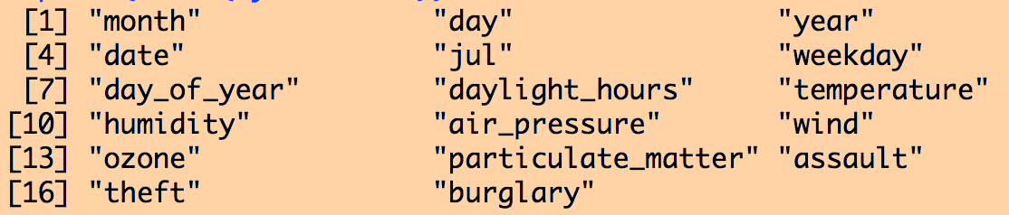
print(names(mydat))

####################################################
# subset the data into a training and testing
# sample
####################################################
mydat_train = subset(mydat,year<=2006)
mydat_test = subset(mydat,year>2006)

This code divides the data frame into two halves.

The contents of the data frame are:

Now let’s fit a model to the daily number of assaults in the training data that includes all the weather variables, and pollution variables, and also includes weekday as a factor, number of daylight hours, and linear trend in time:

####################################################
# fit a model with trend, weekday, daylight
# hours, weather variables, and air pollution
# variables
####################################################
model_train = lm(assault~date+
 factor(weekday)+
 daylight_hours+
 temperature+
 humidity+
 wind+
 air_pressure+
 ozone+
 particulate_matter,
 data=mydat_train)

print(summary(model_train))
print(AIC(model_train))

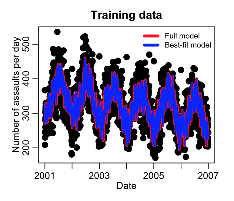
mult.fig(4,main="Chicago crime data 2001 to 2012")
plot(mydat_train$date,
 mydat_train$assault,
 cex=2,
 xlab="Date",
 ylab="Number of assaults per day",
 main="Training data")
lines(mydat_train$date,model_train$fit,col=2,lwd=4)

Not all of the potential explanatory variables were perhaps needed in the fit.  Let’s check by doing model selection using stepAIC():

####################################################
# now do model selection based on the training data
####################################################
require("MASS")
sub_model_train = stepAIC(model_train)

print(summary(sub_model_train))
print(AIC(sub_model_train))
lines(mydat_train$date,sub_model_train$fit,col=4,lwd=2)
legend("topright",
 legend=c("Full model","Best-fit model"),
 col=c(2,4),
 lwd=4,
 bty="n",
 cex=0.8)

This produces the following plot.  Which variables got dropped from the fit?

Now let’s see how well this fitted model predicts the patterns in the testing data set.  We use the R predict() function to do this:

####################################################
# now predict the results for the test data
# and overlay them
####################################################
y = predict(sub_model_train,mydat_test)

plot(mydat_test$date,
 mydat_test$assault,
 cex=2,
 xlab="Date",
 ylab="Number of assaults per day",
 main="Testing data")
lines(mydat_test$date,y,col=3,lwd=2)

 

This code produces the plot:

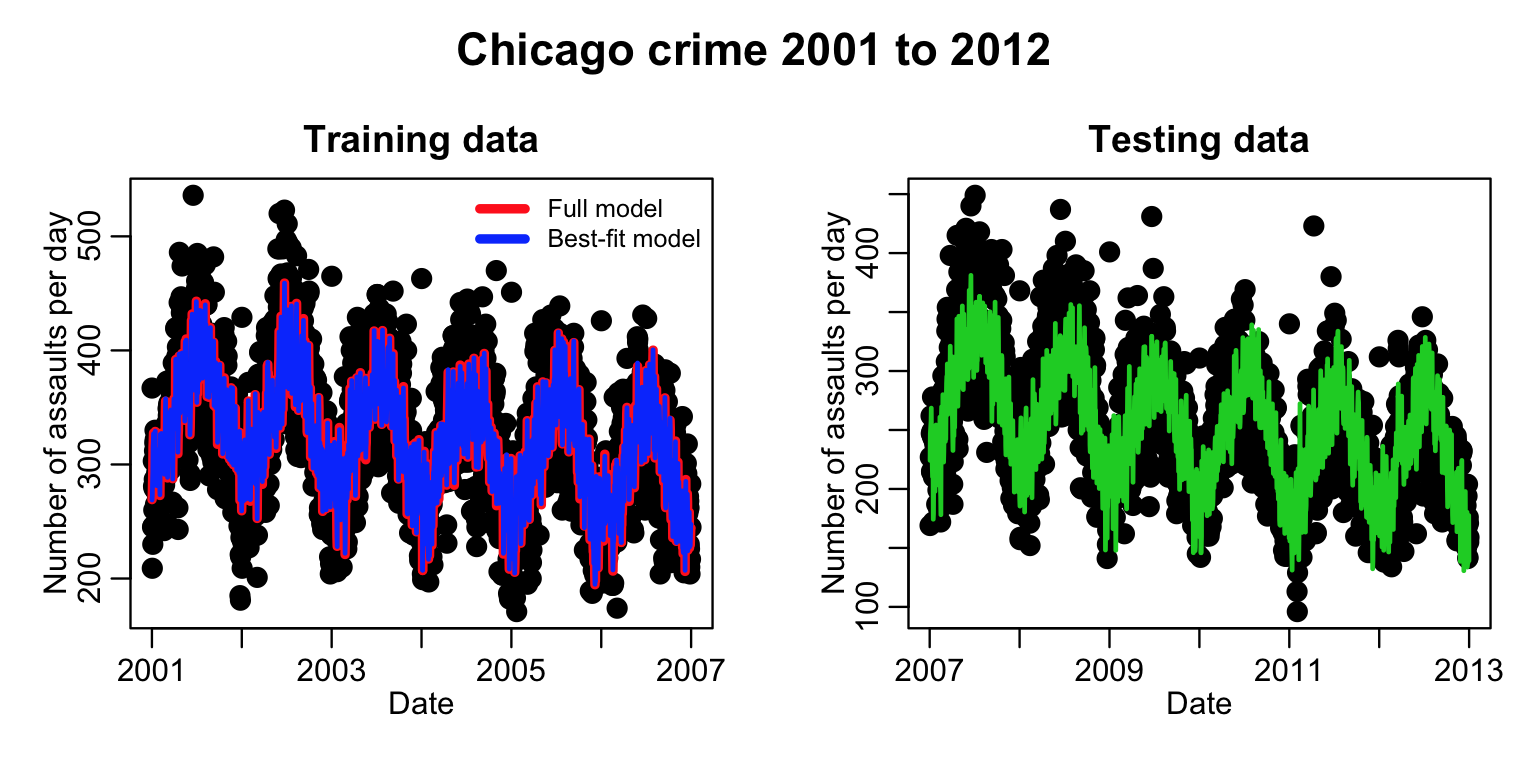
Well…. just visually, the model appears to do a reasonable job of predicting the next six years of data.  But what we need is a quantification of how much better it fits compared to the null hypothesis model (which is just fitting a flat line).

The following code fits the null model to the test data, then “fits” the extrapolated prediction from the training model as an offset() with no intercept term.  This isn’t really a fit at all, in the sense that it has no coefficients, but it does allow us to extract the AIC, and compare it to the AIC of the null model.  If the extrapolated data fits the test data better than the null hypothesis model, the AIC will be smaller:

####################################################
# fit the null model to the test sample
# (just the mean)
# In order to compare this to how well the
# extrapolation of the training sample fits the
# data, "fit" that model as offset(y) but without
# an intercept (-1 on the RHS forces the fit
# to not include an intercept term)
####################################################
null_fit_test = lm(mydat_test$assault~1)
comparison_training_fit_test = lm(mydat_test$assault~offset(y)-1)

print(AIC(null_fit_test))
print(AIC(comparison_training_fit_test))

Does the extrapolated fit do a better job of fitting the data than the null model?

Example of split sample validation with Poisson likelihood fit

In the previous example, we used Least Squares regression to fit count data.  Even though there were plenty of assaults per day (and thus the Poisson distribution approaches the Normal), this still isn’t the best method to be using with count data.  It would be better if we used Poisson likelihood fits with the glm() method instead:

####################################################
####################################################
# now do a Poisson likelihood fit instead
####################################################
model_train = glm(assault~date+
 factor(weekday)+
 daylight_hours+
 temperature+
 humidity+
 wind+
 air_pressure+
 ozone+
 particulate_matter,
 data=mydat_train,
 family="poisson")

print(summary(model_train))
print(AIC(model_train))

plot(mydat_train$date,
 mydat_train$assault,
 cex=2,
 xlab="Date",
 ylab="Number of assaults per day",
 main="Training data")
lines(mydat_train$date,model_train$fit,col=2,lwd=4)

sub_model_train = stepAIC(mod)
print(summary(sub_model_train))
print(AIC(sub_model_train))

lines(mydat_train$date,sub_model_train$fit,col=4,lwd=2)
legend("topright",
 legend=c("Full model","Best-fit model"),
 col=c(2,4),
 lwd=4,
 bty="n",
 cex=0.8)

Let’s predict the results for the test data, and then get the AIC of the model with the predicted results and compare it to the null hypothesis model of just a flat line.  Note that Poisson regression has a log-link, thus you have to make sure you take the log of the predicted values in the offset() function on the RHS of the fit equation!

####################################################
# now predict the results for the test data
# and overlay them
####################################################
y = predict(sub_model_train,mydat_test,type="response")

plot(mydat_test$date,
 mydat_test$assault,
 cex=2,
 xlab="Date",
 ylab="Number of assaults per day",
 main="Testing data")
lines(mydat_test$date,y,col=3,lwd=2)

####################################################
# fit the null model to the test sample
# (just the mean)
# In order to compare this to how well the
# extrapolation of the training sample fits the
# data, "fit" that model as offset(y) but without
# an intercept (-1 on the RHS forces the fit
# to not include an intercept term)
####################################################
null_fit_test = glm(mydat_test$assault~1,family="poisson")
comparison_training_fit_test = glm(mydat_test$assault~offset(log(y))-1,family="poisson")

print(AIC(null_fit_test))
print(AIC(comparison_training_fit_test))

This example code produced the following plot:

Note the fit results look quite similar to the Least Squares fits we did above.  This is because there were quite a few assaults per day, and thus the Poisson distribution was in the Normal regime.  We probably could have gotten away with a Least Squares analysis, but it is always good to be rigorous and use the most appropriate probability distribution.

Monte Carlo methods for model validation

Especially for time series data, it is always a good idea to show that a model that is fit to the first half of the time series has good predictive power for the second half, which is what we did in the above example.  More generally, however, it is a good idea to show that a model trained on one half of the data randomly selected from the sample usually has good predictive power for the second half.

If you randomly select half the data many times, train the model, then compare its predictive capability to the second half, you can see how often the model prediction for the second half has better predictive power than just a null model.

The issue of model selection starts to get a bit tricky, however, because the terms that might be selected for one randomly selected training sample might not be exactly the terms selected for a differently randomly selected samples.

One thing you can do is do the model selection process on the full sample.  Then do a repetitive process where you fit that model to the randomly selected training sample, and see how often the extrapolated model provides a better prediction for the remaining data.

In the following code, we use the R formula() function to extract the model terms for the selected model that is produced by the stepAIC function:

####################################################
####################################################
# first fit to the full sample, and
# select the most parsimonious best-fit model
####################################################
model = glm(assault~date+
 factor(weekday)+
 daylight_hours+
 temperature+
 humidity+
 wind+ 
 air_pressure+
 ozone+
 particulate_matter,
 data=mydat,
 family="poisson")

sub_model = stepAIC(train_fit)
sub_formula = formula(sub_model)
cat("\n")
cat("The formula of the sub model is:\n")
print(sub_formula)

 

Now do many Monte Carlo iterations where we fit this sub model to one half of the data, randomly selected, and test it on the second half:

####################################################
# now do many iterations, randomly selecting
# half the data for training the sub model, and
# testing on the remaining half
####################################################
vAIC_null = numeric(0)
vAIC_comparison = numeric(0)
for (iter in 1:100){
 cat("Doing iteration:",iter,100,"\n")

iind = sample(nrow(mydat),as.integer(nrow(mydat)/2))
 mydat_train_b = mydat[iind,]
 mydat_test_b = mydat[-iind,]

sub_model_train_b = glm(sub_formula,data=mydat_train_b,family="poisson")

y = predict(sub_model_train_b,mydat_test_b,type="response")
 null_fit_test = glm(mydat_test_b$assault~1,family="poisson")
 comparison_training_fit_test = glm(mydat_test_b$assault~offset(log(y))-1,family="poisson")

vAIC_null = c(vAIC_null,AIC(null_fit_test))
 vAIC_comparison = c(vAIC_comparison,AIC(comparison_training_fit_test))
}

f = sum(vAIC_comparison<vAIC_null)/length(vAIC_null)
cat("The fraction of times the predicted model did better than the null:",f,"\n")

 

The R bootStepAIC package

R has a packages called bootStepAIC.  Within that package, there is a method called boot.stepAIC(model,data,B) that takes as its arguments an lm or glm model object previously fit to the data.  It also takes as its argument the data frame the data were fit to, and a parameter, B, that states how many iterations should be done in the procedure.

If there are N points in the data samples, what boot.stepAIC does is randomly samples N points from that data, with replacement to create what is known as a “bootstrapped” data sample.  Thus, the sampled data set looks somewhat like the original data set, but with some duplicated points, and some points missing.  For large data samples, the bootstrapped data set will overlap the original data set by a fraction (1-1/e)~0.632

For the bootstrapped data set, the boot.stepAIC performs the stepAIC procedure, to determine which explanatory variables form the most parsimonious model with best explanatory power.  It then stores the information of which variables were chosen.

Then it samples another bootstrapped sample and repeats the  procedure.  And again, and again, and again, until the iteration limit, B, has been reached (the default is B=100 iterations of this Monte Carlo bootstrapping procedure).

At the end of the procedure, the bootstepAIC method tells you how often each explanatory variables was selected in the stepAIC procedure.  An explanatory variable that was selected 100% of the time, for example, is likely to have good explanatory power for independent data sets.  If it only was selected 20% of the time, for example, it is unlikely to have good general predictive power, and is likely reflecting over-fitting to statistical fluctuations in your particular data.

require("MASS")

model = glm.nb(assault~date+
 factor(weekday)+
 daylight_hours+
 temperature+
 humidity+
 wind+
 air_pressure+
 ozone+
 particulate_matter,
 data=mydat)
 
if (!"bootStepAIC"%in%installed.packages()[,1]){
 install.packages("bootStepAIC")
}
require("bootStepAIC")
b = boot.stepAIC(model,mydat,B=25)
print(b)

This produces the following output (amongst other things):

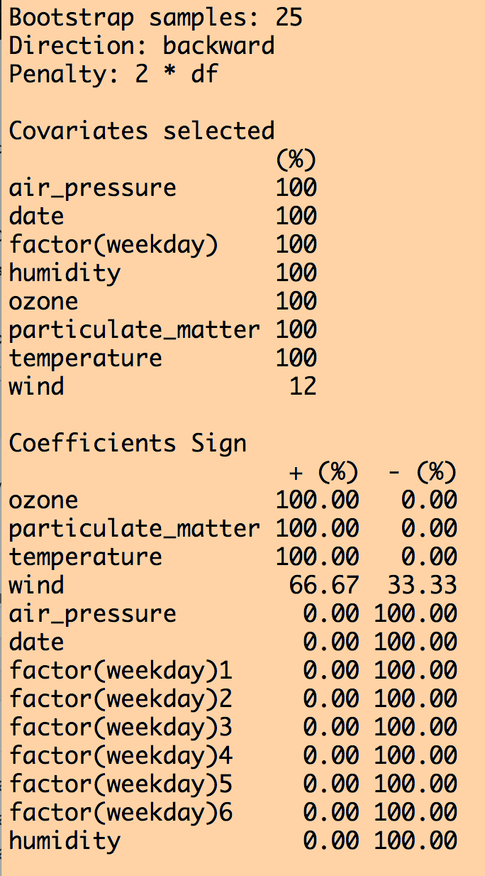
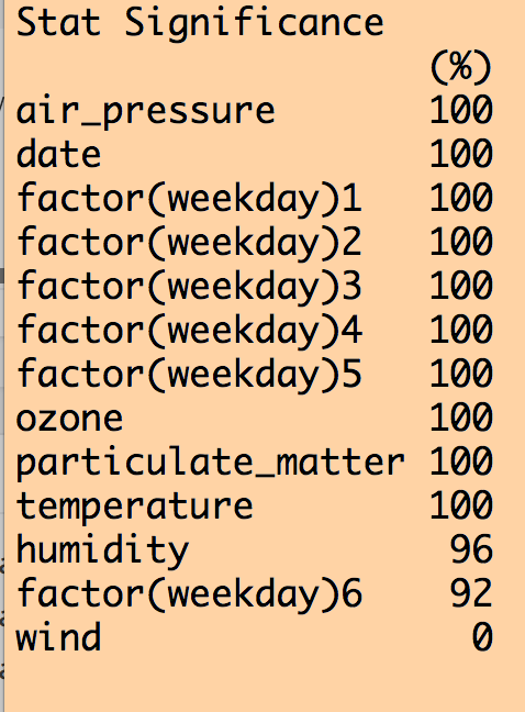
We can see that all variables except for wind were selected 100% of the time out of the 25 iterations.  Except for wind, the coefficient for the other explanatory variables was either consistently +’ve or consistently -‘ve 100% of the time.  However, when we look at how often each variable was significant to p<0.05 in the fits, humidity was not always significant, and wind never was (ignore the weekday=6 factor level… if one of the levels is always significant, you should keep that factor).

How to proceed from here is largely arbitrary… If you use large B (use at least B=100… I used a smaller value of B here just to make the code run faster) you of course should keep all variables that are selected 100% of the time that were always significant to p<0.05, and were consistent in the sign of the their influence.  As for whether or not you relax the selections to include variables that were significant at least 80% of the iterations (for example), that is up to you.  But because this is an arbitrary selection, it’s a good idea to do a cross-check of the robustness of your analysis conclusions to an equally reasonable selection, like 70%, or 90%.  Or, rely on the selection used in past papers on the subject;  for example, this paper recommends a 60% selection.  The former is preferable, but the latter will get through review.

To see how this procedure is talked about in a typical publication, see this paper.  Specifically, pay attention to the second to last paragraph, where it is made clear that the model validation and robustness crosschecks are an important part of the analysis, and the middle and bottom of page 8 where the bootstrapping method and model validation methods are described.

This paper gives more information about bootstrapping methods. And this book is a good one to cite on the topic of the importance of model validation.