In this module, we will discuss the graphical Monte Carlo parameter optimisation procedure using Uniform random sampling of the parameter hypotheses, and compare and contrast this method with the graphical Latin hypercube method.

Once you have chosen an appropriate goodness-of-fit statistic comparing your model to data, you need to find the model parameters that optimise (minimise) the goodness-of-fit statistic.  The graphical Monte Carlo Uniform random sampling method is a computationally intensive “brute force” parameter optimisation method that has the advantage that it doesn’t require any information about the gradient of the goodness-of-fit statistic, and is also easily parallelizable to make use of high performance computing resources.

In this module, we discussed a related method, graphical optimisation with Latin hypercube sampling. With Latin hypercube sampling, you assume that the true parameters must lie somewhere within a hypercube you define in the k-dimensional parameter space.  You grid up the hypercube with M grid points in each dimension.  In the center of each of the M^k points, you calculate the goodness-of-fit statistic.  With this method you can readily determine the approximate location of the minimum of the GoF.  Because nested loops are involved, with use of computational tools like OpenMP, the calculations can be readily parallelized to some degree.  However, if the sampling region of the hypercube is too large, you need to make M large to get sufficiently granular estimate of the dependence of the GoF statistic on the parameters.  Several iterations of the procedure are usually necessary to narrow down the appropriate sampling region.

If you make the sampling range for each of the parameters large enough that you are sure the true parameters must lie within those ranges, with this method you can be reasonably sure that you are finding the global minimum of the GoF, rather than just a local minimum.  This is important, because very often in real epidemic or population data, there are often local minima in GoF statistics.

Because it is difficult to parallelise Latin hypercube sampling, and there is discrete granularity in the sampling, a method which is preferable is randomly Uniformly sampling the parameters over a range.  The method is easy to implement, and easy to parallelise. With this method, parameter hypotheses are randomly sampled from Uniform distributions in ranges that would be expected to include the best-fit values.  The goodness-of-fit statistic is calculated for a particular set of hypotheses, and along with the hypotheses stored in vectors.  The procedure is repeated many, many times, and then the goodness-of-fit statistic is plotted versus the parameter hypotheses to determine which values appear to optimise the GoF statistic.

Example: fitting to simulated pandemic influenza data

We’ll use as example “data” a simulated pandemic flu like illness spreading in a population, with true model:

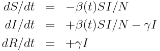
with seasonal transmission rate

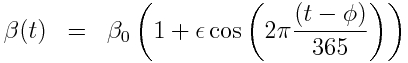
The R script sir_harm_sde.R uses the above model with parameters 1/gamma=3 days, beta_0=0.5, epsilon=0.3, and phi=0. One infected person is assumed to be introduced to an entirely susceptible population of 10 million on day 60, and only 1/5000 cases is assumed to be counted (this is actually the approximate number of flu cases that are typically detected by surveillance networks in the US). The script uses Stochastic Differential Equations to simulate the outbreak with population stochasticity, then additionally simulates the fact that the surveillance system on average only catches 1/5000 cases. The script outputs the simulated data to the file sir_harmonic_sde_simulated_outbreak.csv

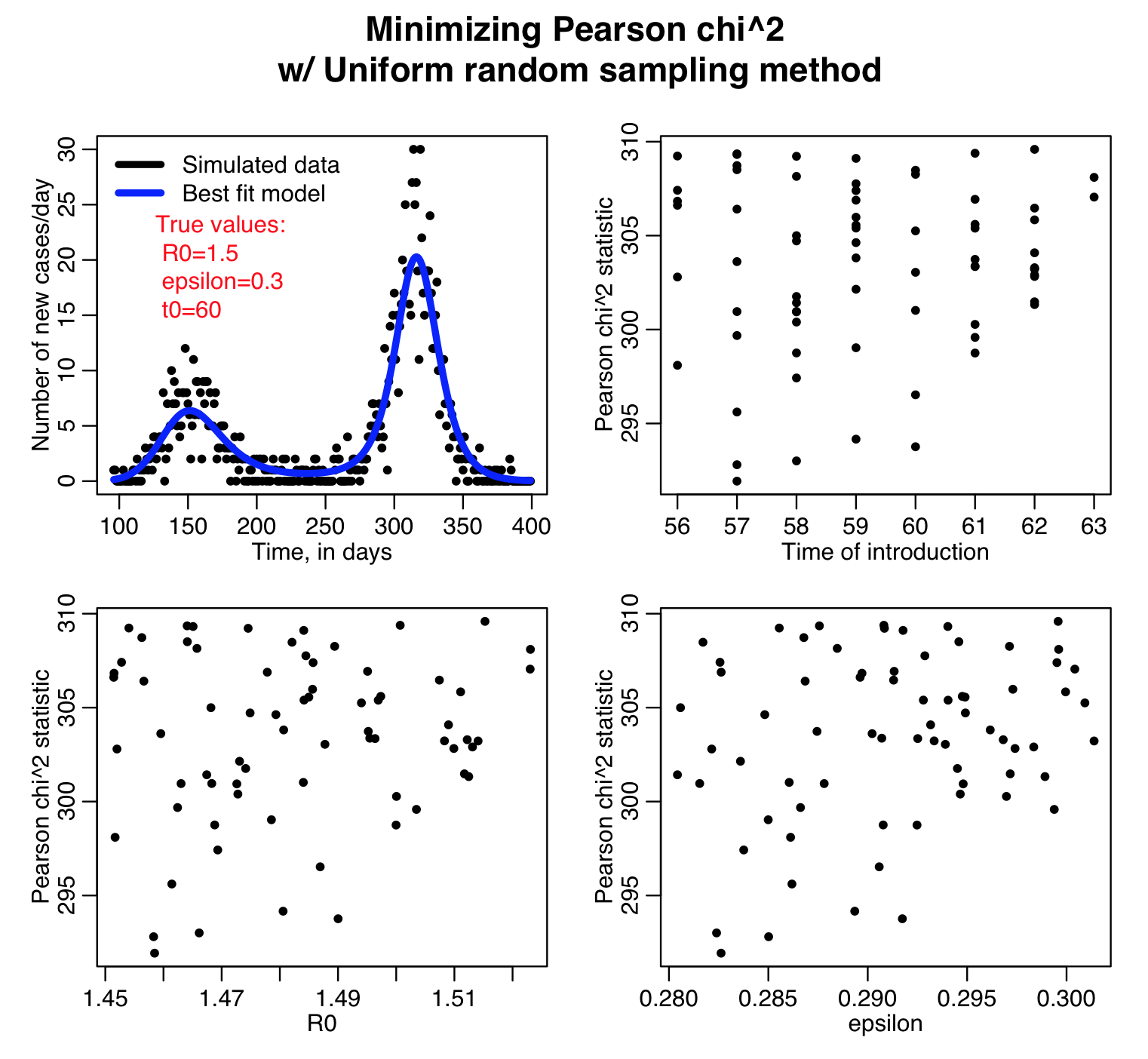
The R script sir_harm_uniform_sampling.R uses the parameter sweep method to find the best-fit model to the simulated pandemic data in sir_harmonic_sde_simulated_outbreak.csv.  Recall that our simulated data and the true model looked like this:

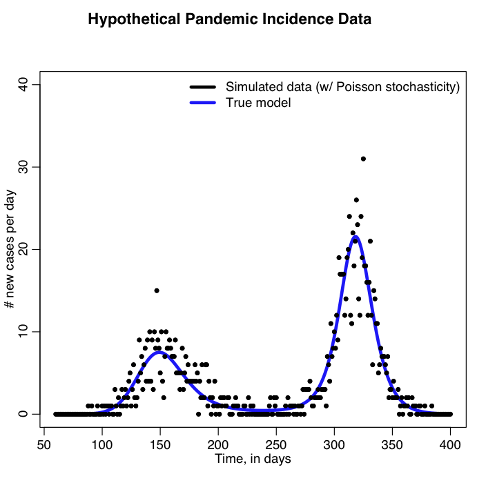
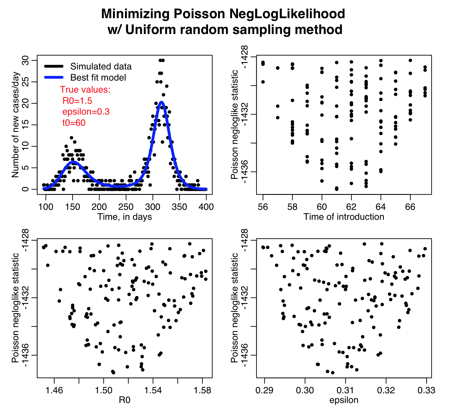
The sir_harm_uniform_sampling.R script randomly Uniformly samples the parameters R0, t0, and epsilon over many iterations and calculates three different goodness-of-fit statistics (Least squares, Pearson chi-squared, and Poisson negative log-likehood).  Question: this is count data… which of those GoF statistics are probably the most appropriate to use?

Here is the result of running the script for 10,000 iterations, sweeping R0, the time of introduction t0, and epsilon parameters of our harmonic SIR model over certain ranges (how did I know which ranges to use? I ran the script a couple of times and fine-tuned the parameter ranges to ensure that the ranges actually contained the values that minimized the GoF statistics, and that the ranges weren’t so broad that I would have to run the script for ages to determine a fair approximation of the best-fit values).  Question: based on what you see in the plots below do you think 10,000 iterations is enough?  Also, do all three GoF statistics give the same estimates for the best-fit values of the three parameters? Which fit would you trust the most for this kind of data?

This method is known as the “graphical Monte Carlo method”.  “Graphical” because you plot the goodness-of-fit statistic versus the parameter hypotheses to determine where the minimum is, and “Monte Carlo” because parameter hypotheses are randomly sampled.

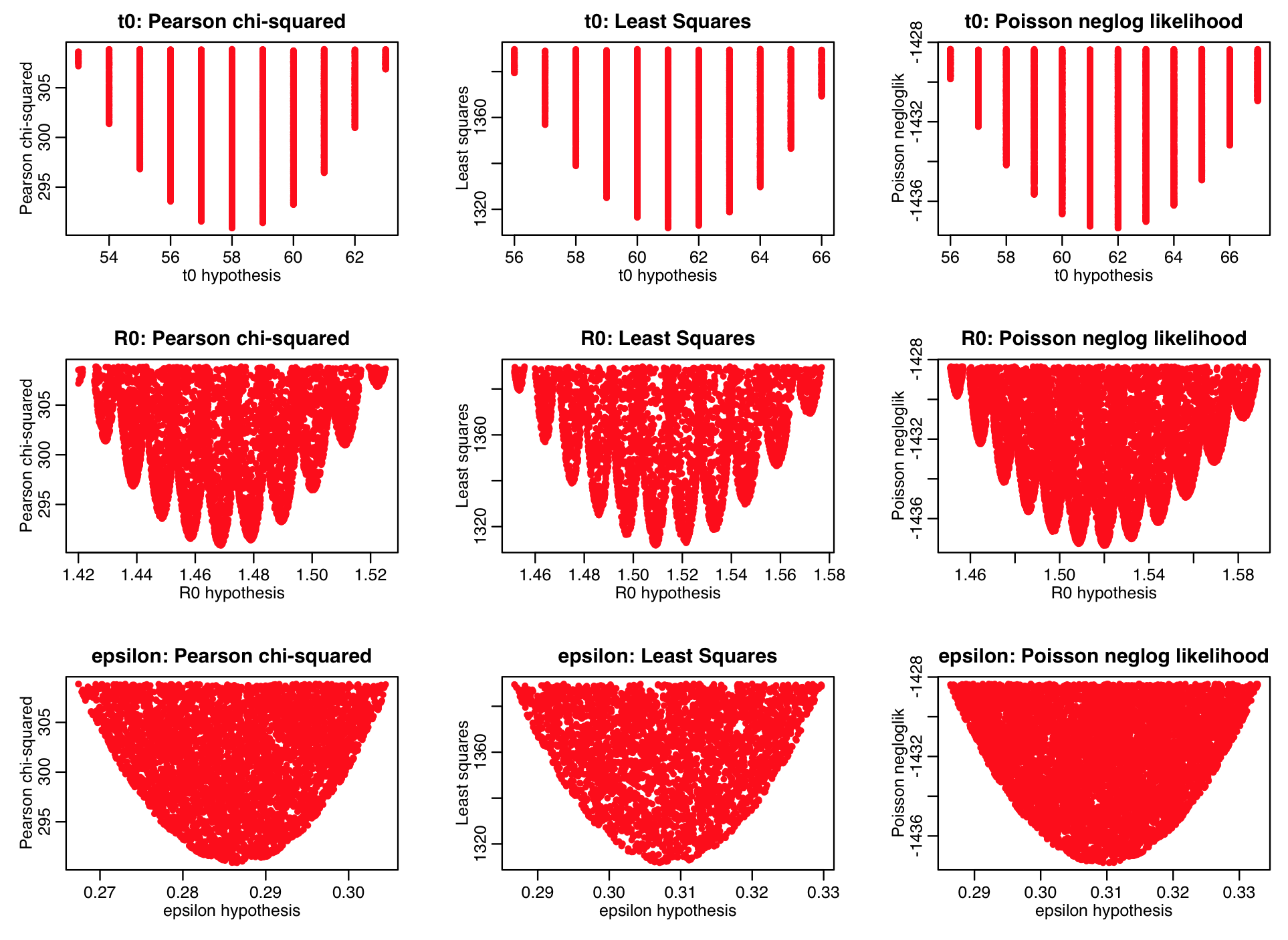
The uniform random sampling method is easily parallelizable to make use of high performance computing resources, like the ASU Agave cluster, or NSF XSEDE resources.

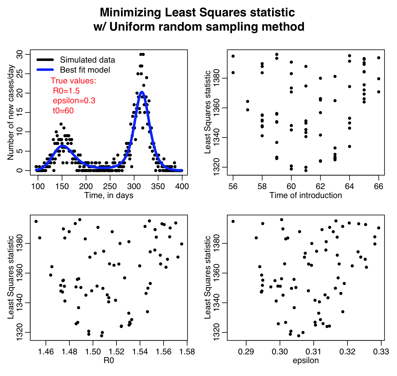
Here is a summary of the results of running the sir_harm_uniform_sampling.R script in parallel using the ASU Agave high performance computing resources (note that the density of points in the plot below are what you are aiming to achieve when using the graphical Monte Carlo procedure… the plots above are too sparse to reliably estimate the best-fit parameters and their uncertainties!).  Note that the Pearson chi-squared, least squares, and Poisson negative log likelihood statistics all predict somewhat different best-fit parameters.  We were fitting to count data… which of these goodness of fit statistics is likely the most appropriate?

In addition to being easily parallelisable, the graphical Monte Carlo method with Uniform random sampling also has the advantage that Bayesian priors on the model parameters are trivially applied post-hoc to the results of the parameter sampling.