
When doing Least Squares or likelihood fits to data, sometimes we would like to compare two models with competing hypotheses. In this module, we will discuss the statistical methods that can be used to determine if one model is significantly statistically favoured over another.
In this past analysis, my colleagues and I examined mass killings data in the US, and fit the data with a model that included a contagion effect, and another model that included temporal trends but no contagion effect. Because the data were count data (number of mass killings per day), we used a Negative Binomial likelihood fit.
And in this past analysis, which was an AML 612 class publication project, we examined data from a norovirus gastrointestinal disease outbreak aboard a cruise ship, and fit the data with a model that included both direct transmission, and transmission from contaminated surfaces in the environment. We also fit a model with just direct transmission, and a model with just environmental transmission. Again, because the data were count data (number of cases per day), we used a Negative Binomial likelihood fit.
In this past analysis, which was also an AML 612 class publication project, we examined US Twitter data and Google search trend data related to sentiments expressing concern about Ebola during the virtually non-existent outbreak of Ebola in the US in 2014. We fit the data with a mathematical model of contagion that used the number of media reports per day as the “vector” that sowed panic in the population, and included a “recovery/boredom” effect where after a period of time, no matter how many news stories run about Ebola, people lose interest in the topic. We compared this to a simple regression fit that did not include a boredom effect.
What helped to make these analyses interesting and impactful was the exploration of what dynamics in the model had to be there in order to fit the data well. When you have the skill set to fit a model to data with the appropriate likelihood statistic and estimate model parameters and uncertainties, it opens up a wide range of interesting research questions you can explore… you fit the model to the data as it is today, and then using that model you can explore the effect of control strategies. However, if you also add in the ability to make statements about which dynamical systems fit the data “better” than alternate modelling hypotheses, you’ll find there is a lot of very interesting low-hanging research fruit out there.
For the purposes of the following discussion, we will assume that we are fitting to our data using a negative log-likelihood statistic (recall that the Least Squares statistic can be transformed to the Normal negative log-likelihood statistic).
Likelihood ratio test for nested models
When two models are “nested” meaning that one has all the dynamics of another (ie: all the dynamics of a simpler “null model”, plus one or more additional effects), we can use what is known as the likelihood ratio test to determine if the more complex model fits the data significantly better. To do this, first calculate the best-fit negative log-likelihood of the null model (the simpler model):
x_0=-log(L_0)
Then calculate the best-fit negative log-likelihood of the more complex model:
x_1=-log(L_1)
The likelihood ratio test is based on the statistic lambda = -2*(x_1-x_2). If the null model is correct, this test statistic is distributed as chi-squared with degrees of freedom, k, equal to the difference in the number of parameters between the two models that are being fit for. This is known as Wilk’s theorem.
If the null hypothesis is true, this means that the p-value
p=1-pchisq(lambda,k) Eqn(1)
should be drawn from a uniform distribution between 0 and 1.
If the p-value is very small, it means the null hypothesis model is dis-favoured, and we accept the alternate hypothesis that the more complex model is favoured. Generally, a p-value cutoff of p<0.05 is used to reject a null hypothesis.
Note that more complex models generally fit the data better than a simpler nested model (ie: the minimum value of the negative log-likelihood statistic will be smaller). This is because the more complex model has more parameters, and those extra parameters give the model more wiggle room to fit to variations in the data. But the problem is that more parameters also increases the uncertainty on all the parameter estimates; so, yes… it might give a lower negative log-likelihood, but there is a cost to be paid for that in the number of parameters you had to add in. The more parameters you add in, the more you are at risk of “over-fitting” to statistical fluctuations in the data, rather than trends due to true underlying dynamics.
The Wilk’s likelihood ratio test in effect penalizes you for the number of extra parameters you are fitting for (that k in Eqn 1 above). The higher k is, the lower the best-fit negative log-likelihood for the more complex model has to be in order for the null model to be rejected.
Example
One example of the kind of research question that can be answered using this methodology: when fitting to data for a predator-prey system (say, coyotes and rabbits), we can examine whether or not a Holling type II model fits the data significantly better than a Holling type I model. In the Holling type I model, the number of prey consumed, Y, is a linear function of the density of prey, X, the discovery rate, a, and the time spent searching, T:
Y = a*X*T Eqn(2)
In a Holling type II model, the relationship is
Y = a*X*T/(1+a*b*X) Eqn(3)
Note that the Holling type I model is nested within the Holling type II model when b=0, and thus a likelihood ratio test can be used to determine if one model fits the data significantly better. The Holling type II model has one extra parameter being fitted for compared to the Holling type I model.
For example, if our “null” Holling type I model when fit to the data with b=0 yields a best-fit negative log-likelihood of x_0=-log(L_0)=900, and our “alternate” Holling type II model yields a best-fit negative log-likelihood of x_1=-log(L_1) = 898.5, we would calculate the negative log test statistic as lamba = -2*(x_1-x_0)=2*1.5=3. If the null hypothesis is true, then lambda should be distributed as chi-squared with degrees of freedom, k, equal to the difference in the number of parameters between the two models (in this case, k=1, because the only difference in the parameters between the two models is the addition of the parameter b). Thus, the test is
pvalue_testing_null=1-pchisq(lambda,difference_in_degrees_of_freedom)
pvalue_testing_null=1-pchisq(3,1)
which yields pvalue_testing_null=0.083. Thus in this case, we would say there is no statistically significant evidence that the Holling type II model fits the data better than the Holling type I model. This doesn’t mean, btw, that the Holling type II model is “wrong” and the Holling type I model is “right”. It simply means that based on these particular data, there is no statistically significant difference. If you had more data, it increases your sensitivity to detecting differences in the dynamics.
If, for example, you fit the two models to another, larger, data set, and find x_0=532 and x_1=521, then in this case
pvalue_testing_null=1-pchisq(-2*(521-532),1)
and we get pvalue_testing_null=2.7e-6, which is very small indeed, and we conclude that the Holling type II model fits the data significantly better. In a paper, we would state these results along these lines: “The Negative Binomial negative log-likelihood best-fit statistics for the Holling type I and Holling type II models were 531 and 521, respectively. The likelihood ratio test statistic has p-value<0.001, thus we conclude the dynamics of the Holling type II model appear to be favoured over those of the type I model.”
What to do if the models being compared aren’t nested
In all of the examples above, we assumed that the models were nested: for example, in the contagion in mass killings analysis, the model without contagion but just with temporal trends was nested within the model with contagion and temporal trends. In the norovirus analysis, the models with just direct transmission, and just environmental transmission, were nested in the model that contained both effects.
But what if we are trying to compare two plausible models that aren’t nested? In that case, we can use the Aikake Information Criterion (AIC) statistic, which is twice the best-fit negative log-likelihood, plus two times the number of parameters being fit for, q:
AIC = 2*(best-fit neg log likelihood) + 2*q
Note that the AIC statistic penalizes you for the number of parameters being fit for… increasing the number of parameters might help bring the negative log-likelihood down, but it can result in an increase of the AIC.
As an overly general statement, models with low AIC are usually preferred over models with high AIC. In fact, in your Stats 101 journeys, you may have heard that you should simply pick the model with the lowest AIC as being the “best” model. However, it’s not quite that simple. Sometimes, one model might give a slightly lower AIC than another, but that does not mean that it is definitively “better”….
Quantitatively using AIC to compare models
We can use what is known as the “relative likelihood” of the AIC statistics to quantitatively compare the performance of two models being fit to the same data to determine if one appears to “significantly” fit the data better.
To do this, we first must calculate the AIC of the two models. If the negative log-likelihood of model #1 is x_1=-log(L_1), and the negative log-likelihood of model #2 is x_2=-log(L_2), then the AIC statistic for model number 1 is
AIC_1 = 2*x_1 + 2*q_1
where q_1 is the total number of parameters being fitted for in model #1, and the AIC statistic for model #2 is
AIC_2 = 2*x_2 + 2*q_2
where q_2 is the total number of parameters being fitted for in model #2.
Now, find the minimum value of the two AIC statistics,
AIC_min = min(AIC_1,AIC_2)
Then, for each model, calculate the quantity:
B_i=exp((AIC_min-AIC_i)/2)
And then for each model calculate what is known as the “relative likelihood” (see also this paper):
p_i = B_i/sum(B_i)
If one of the models has a relative likelihood p_i>0.95, we conclude it is significantly favoured over the other.
As mentioned above, sometimes people just choose the model that has the lowest AIC statistic as being the “best” model (and in fact this is very commonly seen in the literature), but problems arise when there is only a small difference between the AIC statistics being compared. If they are very close, one model really is not much better than the other. Calculation of the relative likelihood statistic makes that apparent.
You can use AIC statistic to compare nested models, but if the models truly are nested, then the Wilk’s likelihood ratio test is preferred.
AIC Example #1
As an example of the use of AIC statistics to compare models let’s examine our Holling type I/II hypothetical analysis (even though it is a nested model example, and the Wilk’s likelihood ratio test would be the preferred method to compare the models).
If our Holling type I model when fit to the data with parameter b=0 yields a best-fit negative log-likelihood of x_1=-log(L_0)=900 and one parameter is being fit for (the “a” in Equation 2) then the AIC statistic for that model is
AIC_1 = 2*900 + 2*1=1802
If the fit of our Holling type II model yields a best-fit negative log-likelihood of x_2=-log(L_1) = 898.5, when two parameters are being fit for (the “a” and “b” in Equation 3), then the AIC statistic for that model is
AIC_2 = 2*898.5 + 2*2=1801
Thus, the AIC of the Holling type II model looks to be just a little bit lower than that of the Holling type I model. The B statistics for the two models are
B_1 = exp((1801-1802)/2) = 0.606
B_2 = exp(0) = 1
And the relative likelihoods are
p_1 = B_1/(B_1+B_2) = 0.606/1.606 = 0.377
p_2 = B_2/(B_1+B_2) = 1/1.606 = 0.623
Neither of these p_i’s are greater than 0.95, so we conclude that neither model is significantly favoured over the other.
In a paper, we would state these results along the following lines: “The AIC statistics derived from the Holling type I and Holling type II model fits to the data are 1802 and 1801, respectively. Neither model appears to be strongly preferred [1]”.
With reference [1] being:
Wagenmakers EJ, Farrell S. AIC model selection using Akaike weights. Psychonomic bulletin & review. 2004 Feb 1;11(1):192-6.
However, as noted above, because these are actually nested models, a better choice would be Wilk’s test. In practice, you should only use AIC for non-nested models.
AIC Example #2
If our Holling type I model when fit to another set of data with parameter b=0 yields a best-fit negative log-likelihood of x_1=-log(L_0)=532 and one parameter is being fit for (the “a” in Equation 2) then the AIC statistic for that model is
AIC_1 = 2*532 + 2*1=1066
If the fit of our Holling type II model yields a best-fit negative log-likelihood of x_2=-log(L_1) = 521, when two parameters are being fit for (the “a” and “b” in Equation 3), then the AIC statistic for that model is
AIC_2 = 2*521 + 2*2=1046
The AIC of the Holling type II model is lower than that of the Holling type I model. The minimum value of the AIC for the two fits is 1046.
The B statistics for the two models are thus
B_1 = exp((1046-1066)/2) = 4.5e-5
B_2 = exp(0) = 1
And the relative likelihoods are
p_1 = B_1/(B_1+B_2) = 4.5e-5/1.000045 = 4.5e-5
p_2 = B_2/(B_1+B_2) = 1/1.000045 = 0.99996
The relative likelihood of the second model is greater than 0.95, thus we conclude it is significantly favoured.
In a paper we would say “The AIC statistics derived from the Holling type I and Holling type II model fits to the data are 1066 and 1046, respectively. We conclude the Holling type II model is significantly preferred [1].” With reference [1] again being:
Wagenmakers EJ, Farrell S. AIC model selection using Akaike weights. Psychonomic bulletin & review. 2004 Feb 1;11(1):192-6.
AIC Example # 3
The R script example_AIC_comparison.R generates some simulated data according to the model A*exp(B*x)+C with Poisson distributed stochasticity. It then uses the graphical Monte Carlo method to fit a linear model (intercept+slope*x) and the model A*exp(B*x)+C to the simulated data using the Poisson negative log-likelihood as the goodness of fit statistic.
After 50,000 iterations of the Monte Carlo sampling procedure, the script produces the plot:
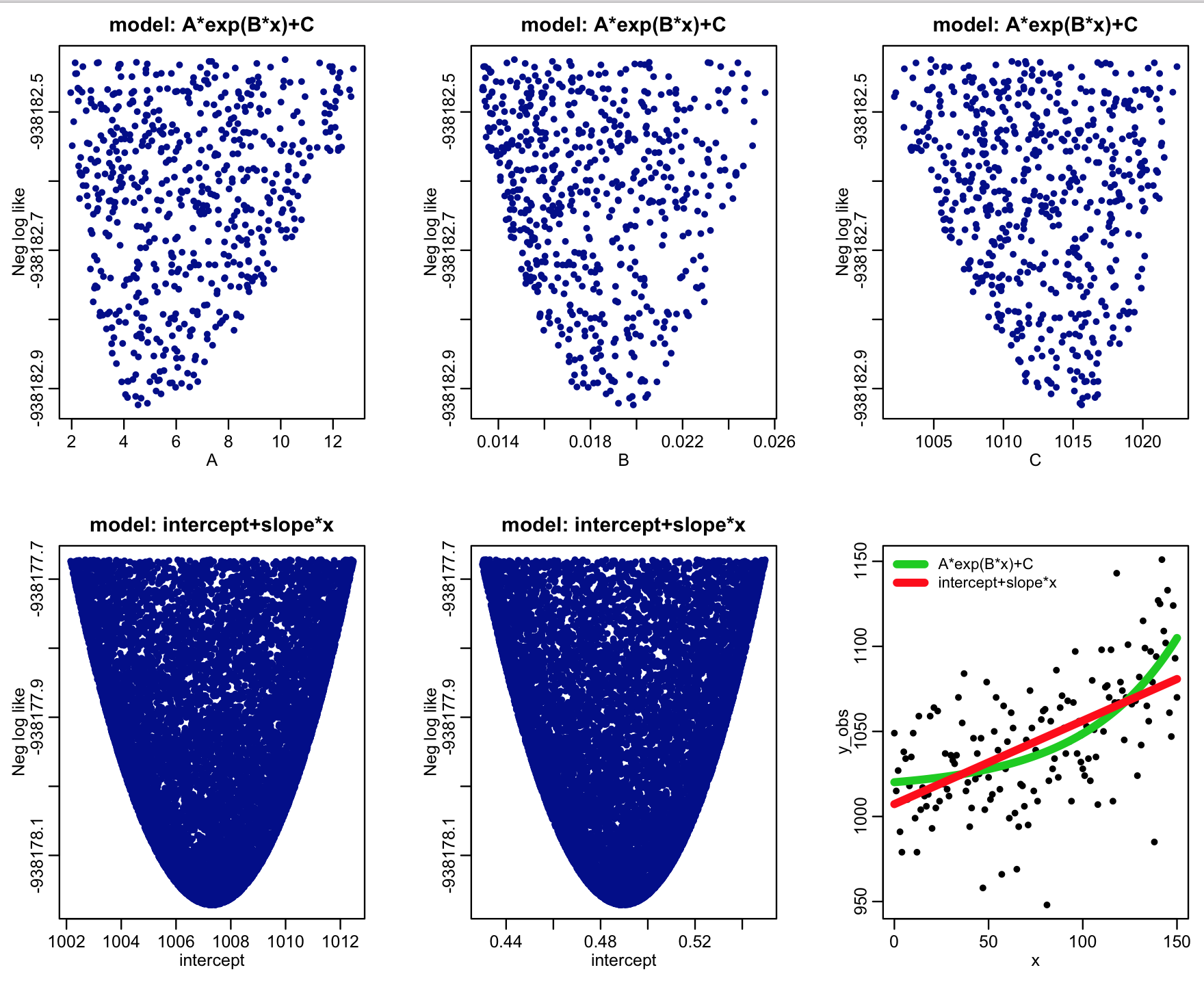
Based on the best-fit negative log likelihoods and the number of parameters being fit for for each model (two for the linear model, and three for the exponential model), the script also calculates the AIC statistic, and the relative likelihoods of the models derived from those statistics.
The script outputs the following:

We see that the relative likelihood of the exponential model (which was actually the true model underlying the simulated data) is significantly favoured over the linear model.
Something to try is instead of using integer values of x from 0 to 150 in the script, use integer values from 0 to 50. You will find with this smaller dataset that there is no statistically significant difference between the two models… there is simply not enough data to make the determination.
