[This post is part of a series of posts on archaeoastronomy using open source software]

In order to calculate where stars rise and set on the horizon at a particular location, we need to know what the horizon looks like at that place… are there mountains along the horizon?  If so, they can substantially change the rise or set azimuth of a star, compared to a flat horizon.

The website HeyWhatsThat allows you to enter the latitude and longitude and elevation of any location on earth, and get the horizon profile. Here is what the screen shot of the input page looks like: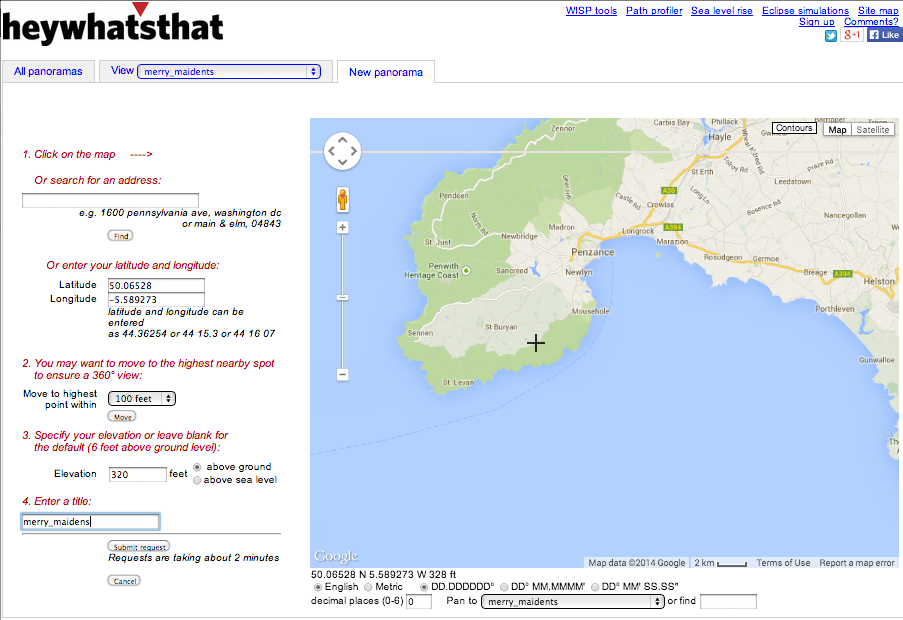

It takes a the website a few seconds to compute the profile (but surprisingly little time actually, considering how complex the calculation is!), and this is what it outputs for the horizon profile for Merry Maidens: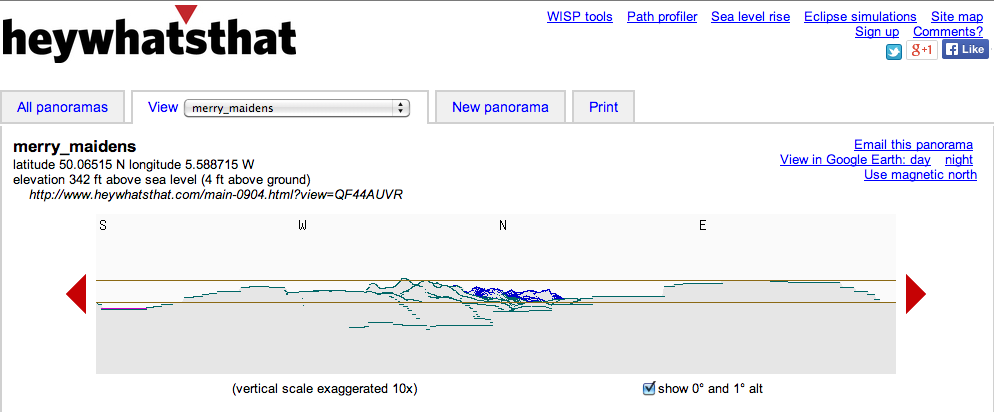

Notice that there is a link on the upper right hand side that says “View in Google Earth: day”.  If you click on the link, it will download a file in kmz format which can be read into Google Earth.  Click on the file once it is downloaded, and Google Earth will show you the “viewshed” from your site.  Here is what it looks like: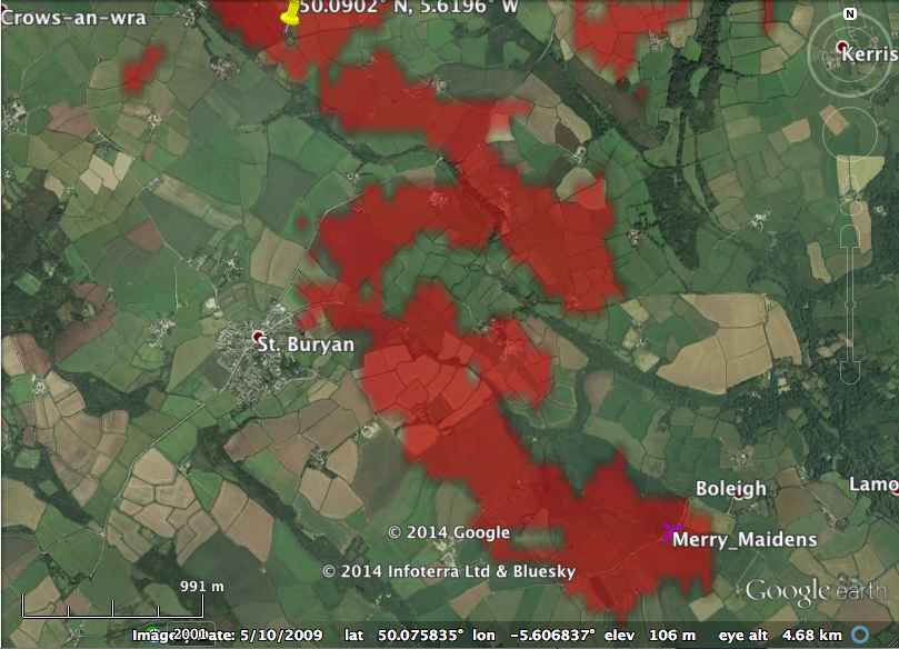

Isn’t that cool? Notice the yellow “push pin” to the upper left.  That is the circle of Boscawen-Un… it thus appears that the Boscawen-Un site is just visible from the Merry Maidens site, even though it is over 3km away.  Here is the viewshed from Boscawen-Un that I downloaded from the Hey What’s That site… you can see that Merry Maidens is also a particular point in the viewshed from Boscawen-Un: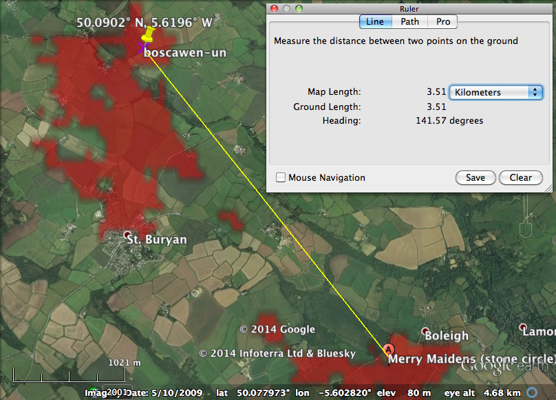

The only problem with HeyWhatsThat is that you cannot download the data for the horizon profile, just the plot, and in order to correct the rise/set azimuths of stars, we need the data for the horizon dip angle vs azimuth.

Calculating horizon dip angle: getting terrain data

We can estimate the horizon profile ourselves by first getting elevation data of points on the terrain of the surrounding area.  In February 2000 the Space Shuttle flew an 11 day mission that conducted a radar topography survey of the Earth.  The Shuttle Radar Tomography Mission (STRM) elevation data were taken in a grid of 90m increments across the surface of the Earth.  The data are available online from the CGIAR Consortium for Spatial Information website. Choose the output format to be ArcInfo ASCII, and then click on the map grid(s) that are close in location to your archaeological site, and download the data.  Copy the srtm .asc files to your working directory.

The R script convert_srtm_raster_to_xyz.R reads in the srtm .asc files associated with the Merry Maidens site, and selects the points within a wide enough window that you include all latitudes and longitudes that are visible from the site (from the HeyWhat’sThat .kmz file that I viewed in Google Earth, it appears that taking +/-0.15 degrees of latitude and longitude from the Merry Maidens site is sufficient).  It then converts to XYZ (x=longitude, y=latitude, z=elevation), and writes the text output to a file long_lat_elev_surrounding_area.txt

In order to ensure that the exact location and elevation data for mountains in the nearby area are included in the data, I often append on to this file the longitude, latitude, and elevation of local mountains.  The ExpertGPS website has lat/long/elev data (elevation given in meters) for most mountains in the US (it appears they define “mountains” as pointy land features over 100m high).  To get the data, select the state, then once on the webpage with the state data, click on “Download a GPX file…”.    In the R script gpx_parse.R I provide the code that reads in a file in GPX format (just modify the file name variable in the script to reflect the name of your GPX data file), and parse the longitude, latitude, and elevation data.  It puts this info into a file <yourfilename>_parsed_lat_long_elev_data.txt.

For instance, I used the gpx_parse.R script to read in the mountain GPX format information for Nevada in the file nv-mountains.txt  The script output the longitude, latitude, and elevation into the file nv-mountains_parsed_lat_long_elev_data.txt

You can just append this file with the mountain data onto the gridded long/lat/elev data you get from the Shuttle Radar Tomography Mission.

Calculating the horizon profile: calculating dip angles

Determining what is visible from a particular location given the data for the surrounding terrain is known as a “viewshed” analysis.  With a viewshed analysis, we begin by calculating the dip angle (from horizontal) needed to (at least in theory) view a particular point on the terrain from our observation location.  I say “at least in theory” because the point may be so far away it is below the horizon because of the Earth’s curvature, or there may be a high mountain in the way blocking the view.  The horizon profile when looking towards a particular bearing on the horizon is determined by the terrain point on that bearing that has the largest dip angle.

The site cosinekitty has a nice online calculator that gives you the dip angle when viewing some lat/long/elev from some other lat/long/elev. Calculating the viewing dip angle is a relatively straightforward application of trigonometry: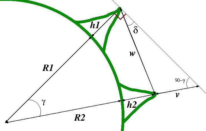

The angle gamma is obtained by first translating the lat/long of the two points in the spherical coordinate system of the sphere of the Earth to Cartesian coordinates:

where R is the radius of the earth. Recall your linear algebra: the cosine of the angle, gamma, is just the dot product of these two vectors, divided by their lengths (in this case, approximately the Earth’s radius, R, because R is much larger than the heights of any mountains).  This yields

Now, take a look at the diagram above… is it obvious to you that the distance, w, between the points can be found by the Law of Cosines?  Thus we have

Now, from the Law of Sines, we can see from the above diagram that we must have

Solving for the dip angle, delta, yields

Notice that I slipped a negative sign in there…that is because delta in this case lies below the observers horizontal plane, and thus is negative. In the file archeoastronomy_libs.R, I give a function dip_angle_lat(lat2,long2,h2,lat1,long1,h1) that calculates the dip angle observing lat2/long2/h2 from lat1/long1/h1.  The function also returns the distance between the two points, and the bearing of the path between them, starting from the observer’s point.

Putting everything together: calculating the horizon profile

To get the horizon profile for the Merry Maidens site, as described above, I began by obtaining  latitude, longitude, and elevation data from the Shuttle Radar Topography Mission, for points in a 90m lat/long grid in the area surrounding the Merry Maidens site.  The long/lat/elevation file I created with this information is in long_lat_elev_surrouding_area.txt

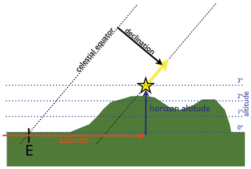
The C++ program calculate_horizon_topography_new.cpp reads in this file, and for a given latitude and longitude calculates the bearing (ie; azimuth), dip angle and distance to each of the gridded lat/long/elev points in the USGS file.  If you are at sea, the dip angle to the horizon is 0.  If you are looking at a mountain from the base of the mountain, your dip angle to the horizon is positive.  If you are standing on top of the mountain looking down, your dip angle to the horizon is negative. Recall from an earlier post that features on the horizon affect the rise/set azimuths of stars, which is the whole point of why we are trying to estimate what the horizon looks like:

The C++ program does more than just calculate the azimuth and dip angle to the gridded USGS points; it also interpolates what the terrain looks like between those points by connecting triangles between triads of nearby points.  Then it randomly samples lat/long/elev on the surface of those triangles. The use of triangles in 3D rendering is very common:

To compile the program on a Unix/Linux/Mac operating system, type

g++ -g -o calculate_horizon_topography_new calculate_horizon_topography_new.cpp

and to run the program type

./calculate_horizon_topography_new.cpp > merry_maidens_azimuth_and_dip_from_interpolated_terrain.txt

The file output of that program, merry_maidens_azimuth_and_dip_from_interpolated_terrain.txt, is too large to link to on this website.  You will need to compile and run the program yourself to get it. Note that the program takes some time to run, because of the computational complexity involved.

Once you have the file, the following R code (horizon_dip_angle.R) reads it in, and examines wedges of 0.1 degree in azimuth, and picks the largest dip angle among the points with azimuth within that wedge… that point will be the horizon point. It does this for azimuth 0 to 360 degrees:

hdat = read.table("merry_maidens_azimuth_and_dip_from_interpolated_terrain.txt",header=T)
g = aggregate(hdat$dip,by=list(as.integer(hdat$azimuth*10)/10),FUN="max")
x = 90-g[[1]]
y = g[[2]]
n = length(y)

r = 5+y # the 5 is just an arbitray number to make the plot look good
xa = r*cos(x*pi/180)
ya = r*sin(x*pi/180)
xb = 5*cos(x*pi/180)
yb = 5*sin(x*pi/180)
a = 6.2
plot(xa[2:(n-1)],ya[2:(n-1)],axes=F,xaxt="n",yaxt="n",xlab="",ylab="",xlim=c(-(a+0.1),(a+0.1)),ylim=c(-(a+0.1),(a+0.1)),main="Horizon profile for Merry Maidens site")
legend("topleft",legend=c("estimated horizon","sea-level horizon"),col=c(1,2),lwd=3,bty="n")
points(xb,yb,col=2,cex=0.2)
arrows(-6,0,6,0,col=4,lwd=3,length=0.25,code=3)
arrows(0,-6,0,6,col=4,lwd=3,length=0.25,code=3)
text(0,a,"N")
text(0,-a,"S")
text(-a,0,"W")
text(a,0,"E")

The code produces this plot (the red line is what the horizon would look like if we were at sea, instead of on hilly land)

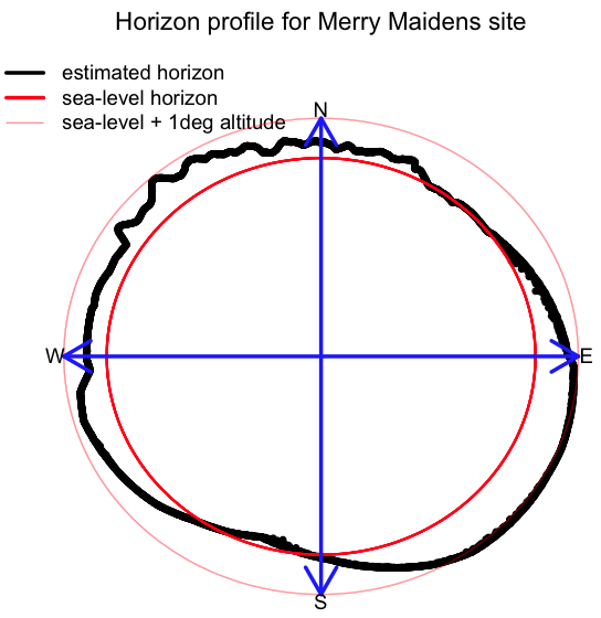
Compare this to the horizon profile calculated by the HeyWhatsThat website:

Pretty close!

If you wanted to run the C++ program for some other archaeological site you are interested in analyzing, first download the Shuttle Radar Tomography Mission data for the area in the near vicinity in latitude and longitude from your site, and put that data in the file long_lat_elev_surrounding_area.txt  (use the viewshed calculated by HeyWhatsThat to aid in selecting the surrounding area… if you select too large an area, the calculation will take a very long time).  Then in the C++ program calculate_horizon_topography_new.cpp  change the lines that set mylatitude, mylongitude, and myelevation to the lat/long/elev (elevation in metres) of your site.  Then compile it and run it.  Note that if your site is in extremely hilly terrain (Machu Picchu, for instance) the 3D interpolation of the terrain can potentially get a bit dodgy if there are nearby large pointy mountains that dominate the horizon, because there is only so much detail that can be captured with terrain that is gridded in 90m increments.  As I described above, one thing I’ve done in those cases is to supplement the long_lat_elev_surrounding_area.txt file with the longitude, latitude and elevation of all mountains in the area.

Correcting for refraction 

The only slightly complicating factor in all of the above is that refraction due to the atmosphere actually means that we can see further than we could if there were no atmosphere:

 

The effect of refraction is to essentially make the point in the distance apparently higher than it actually is.  The apparent change in height is delta_height = k*d^2/(2*R), where k~0.13, d is the distance between the observer and the point, and R is the radius of the earth (in the same units as d).  Notice from the formula that for points close by, refraction does not appear to make them much higher than they actually are, but for distant mountains, this refraction correction can be substantial.  In order to make this correction, simply calculate the distance between the two points, then calculate delta_height, and add it on to the height of the object in all the equations above where we calculate the dip angle. In all the dip angle and horizon profile calculation methods I include in the files archeoastronomy_libs.R and calculate_horizon_topography_new.cpp, the refraction correction is taken into account, and I also account for the oblateness of the Earth.