
[In past modules, we have discussed Markov Chain Monte Carlo methods and Stochastic Differential Equations with Gaussian noise for stochastic modelling of compartmental models. In this module, we will describe how combing the two has the potential to simultaneously optimize computational efficiency and accuracy]
In past modules, we have discussed how Markov Chain Monte Carlo modelling methods are always accurate for stochastic simulation of compartmental models, but not always computationally feasible when the compartment population sizes are large. This is because the time step used in the calculation tends to grow smaller the larger the populations (often in a non-linear way), and thus for very large populations the calculations can get hopelessly bogged down with minuscule time steps.
We discussed how the underlying probability distribution for the number transitioning between compartments in a very small time step is Poisson distributed when using MCMC modelling methods.
To re-iterate what has been pointed out in several past modules on this topic; for compartmental models with exponentially distributed sojourn times, MCMC is always the most exact way to simulate the model. It just is not computationally efficient for large populations.
In another past module, we presented Stochastic Differential Equations with Gaussian noise as a means to address the computational inefficiency of MCMC for larger populations; if we make the time step larger, the number transitioning in that time step approaches the Normal distribution. Thus, with SDE’s we can use a larger time step (and, importantly, a constant time step with no problem), just as long as the time step isn’t so big that the numerical approximation to the first order time derivative of the compartments using Euler’s method is still reasonably accurate.
SDE’s with Gaussian noise are an approximation compared to MCMC methods. But if the population sizes in all compartments are large, it can be a good approximation because the Poisson distribution approaches the Normal distribution when the parameter of the Poisson distribution is large (say, greater than 10 to 25 or so). And with a constant time step, SDE’s can be almost as speedy as calculating the deterministic model.
Because of the approximation made with SDE’s, the problem is that when one of the compartments nears extinction (ie; very small population in the compartment) SDE’s are unreliable because the stochasticity in the change in number in the compartment is now usually no longer in the Normal regime; it is Poisson. And when the probability distribution underlying the stochasticity is Poisson, it is better to be using MCMC methods.
However, from a computational and numerical estimation perspective, there is no reason why you can’t switch between the two as necessary as you step through the model simulation.
Why is this not really discussed in the literature? Because there is a solid body of literature on the mathematical theory underlying MCMC models, and there is a solid body of literature on the theory underlying SDE’s. Or at least I believe that is the reason… stochastic modelling researchers either go solely to an MCMC method, or an SDE method for compartmental models.
But in practice, most compartmental models are complicated enough that there are very few analytic expressions we can derive anyway for the posterior probability distributions for quantities of interest, so we must rely on numerical simulations rather than any theoretical analytic constructs.
And if we are relying on numerical simulations anyway, you might as well optimize them for simultaneous accuracy and computational efficiency*.
Note, however, that combining these two methods really is only necessary when you have simulations where the compartments, within the same simulation, both approach extinction, and at other time points become quite large (which is where the computation starts to bog down). If the number in the compartments is always large, then just use SDE’s. If one or more compartments is always near the edge of extinction, then use MCMC.
How to determine when to switch back and forth between MCMC and SDE
In our algorithm for doing SDE modelling, we need to calculate the state transition rates, because they are needed for the calculation of the G matrix (see this post for all the details).
Recall that the time step needed for on average just one state transition to take place is in the model is delta_t = 1/sum(state transition rates).
The amount of time needed for, say, on average 10 state transitions to take place is 10*delta_t.
And for on average 25 state transitions it is 25*delta_t.
Thus if, for instance, 25*delta_t is greater than the time step being used in the SDE method, it is probably a good time to switch to MCMC and a dynamic time step instead.
And it is easy to do this check on the fly during each step of our simulation, because we must calculate the state transition rates with either method.
Example: SIR model
The R script sir_sde_and_mcmc_mixed.R performs several realisations of a stochastic simulation, switching between MCMC and SDE’s as necessary for a Susceptible Infected Recovered (SIR) type disease circulating in a moderately large population (N=5000).
Every time the script switches between the two methods, it prints out that info to the screen (that is if it switches at all… sometimes it just stays with one method if that was what the most appropriate method was throughout the entire simulation).
The script produces the following plot:
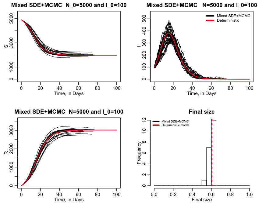
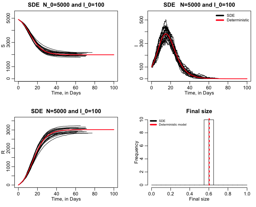
In the script, there is a variable called ltype, that when set to 0 will do mixed SDE+MCMC. When equal to one, it will do only SDE, and when equal to 2 will do only MCMC. If ltype=1, the script produces the plot:
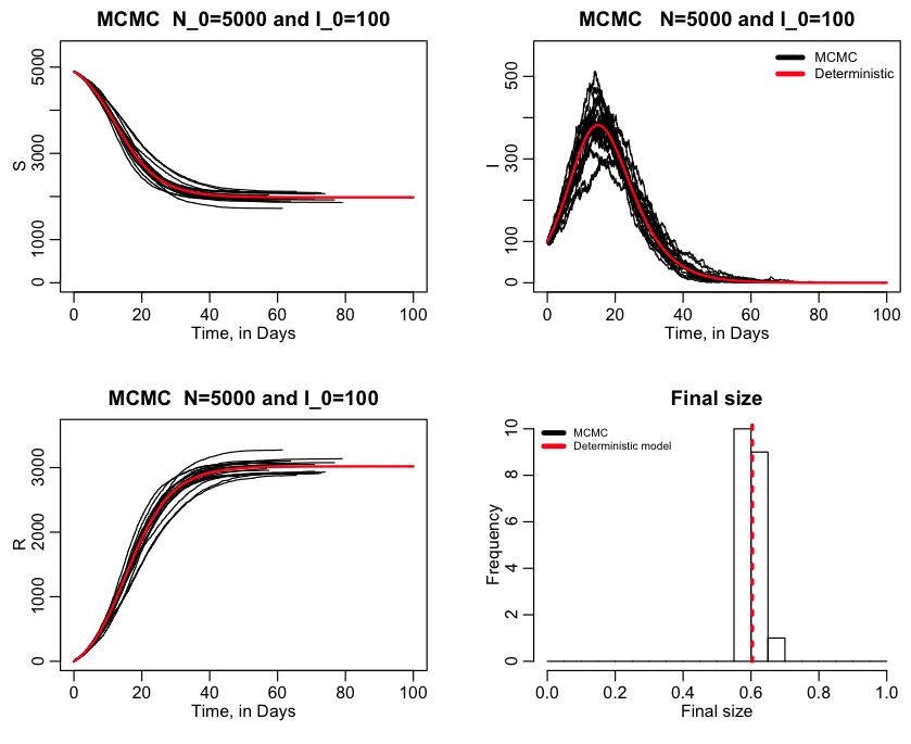
If ltype=2, the script only uses MCMC, and produces the following plot:
How would I describe this mixed method in a publication?
One of the hard things about being early-career and inexperienced is that it is difficult to know how much detail to put into a paper when describing your methodology. If you are writing a paper specifically about developing new advances in theory underlying stochastic modelling methods, you obviously have to go into deep detail.
However, if what you are writing is an applied paper in (for instance) epidemiology or population biology, where you happened to use stochastic modelling methods as part of the analysis, it is actually a bad idea to go into pages of detail. The reviewers are not likely to be stochastic modelling experts, and pages of complex detail will just confuse and potentially intimidate them.
One of the tricks to writing a good applied paper and getting it through review with ease, is to describe your methodology in simple terms, as briefly as possible.
For this particular mixed method, I would state in the Methods and Materials: Mathematical Model section of the paper that, in the interests of computational efficiency and robustness of model estimations, I used Stochastic Differential Equations (and give the equations) as appropriate when the noise in the state transitions was approximately Gaussian at that time step (and give appropriate SDE literature references), switching to MCMC with Poisson noise as appropriate (again, providing appropriate MCMC literature references).
If a reviewer asks for more details, I can then expound on it further if necessary. If the reviewers are OK with the description, just leave it at that.
*This is what happens when you have a non-mathematician applied statistician with a background in high performance computing teach a stochastic modelling course