[In module, students will learn how to aggregate model simulation results into bins of fixed time]
When doing modelling studies, we often wish to compare our model estimates to some data set, either qualitatively or quantitatively.
When obtaining numerical solutions for our model, we will often employ either dynamical time steps in the numerical estimation of the model solution, or small fixed time steps.
However, data almost never comes this way; almost invariably, it is binned into some fixed time step (say, daily, weekly, or monthly) that is different than the time step(s) we use to numerically solve the model. If we wish to qualitatively or quantitatively compare our model results to data, we need to aggregate the results appropriately.
If the model is for disease, the observed quantity is usually the incidence, the number of newly symptomatic cases per unit time (and almost universally, “symptomatic” is taken to mean “infectious”… whether this is a good assumption or not is debatable). In contrast, the prevalence is the fraction of the population in the infectious, I, compartment. For virtually all diseases we do not observe I, unless we go into the population and do seroprevalence studies at regular interviews (which basically never happens). What we observe with the incidence is the number of new cases flowing in to I per unit time.
Take, for example, an SIR model
For this model, the number of new cases flowing into the I compartment per unit time is beta*S*I/N.
In order to aggregate the incidence into fixed time steps T, we would thus sum within each of the fixed time steps the model estimates of delta_t*beta*S*I/N, where delta_t was the time step used in the model calculation. In order for this to work accurately, delta_t must either be much smaller than T, or an integer fraction of T.
In practice, when using a fixed time step to numerically solve the model, one should use an integer fraction of T, T/k, with that fraction being small enough (ie; the integer k being large enough) to ensure accurate numerical solutions. If one is using a dynamical time step calculation, you can instead use delta_t_new = min(delta_t,T/k) to ensure that the time step is never larger than T/k.
The script uses dynamical time steps to calculate the numerical solution. At each time step, it estimates the incidence in that time step, newI=delta_t*beta*S*I/N. It then aggregates the estimated incidence by integer day, much like data would be.
The script produces the following plot (note that you have to install the “weights” library in order to run the script):
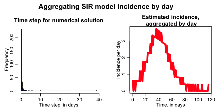
As you can see, the estimated daily incidence curve looks quite choppy. If you look at the histogram of the dynamical time steps, it is clear that a significant fraction of the time, the time step is greater than one day. Thus, the incidence, instead of being spread out over the full more-than-one-day time step, is lumped into one of the days, thus over-estimating the incidence for that day, and under-estimating it for the subsequent day(s).
We can solve this problem, at the cost of a bit of computational inefficiency, by requiring that the dynamical time step be at most some fraction, 1/k, of a day, where the fraction is chosen to be small enough that we don’t get much spill over of incidence day-to-day.
The script has a logical variable lconstrain_time_step, that when equal to 1 ensures that the dynamical time step is, at most, 1/k days with k=10. Set lconstrain_time_step=1 in the sir_aggregate_incidence_by_day.R script, and rerun it. The script then produces the following plot:
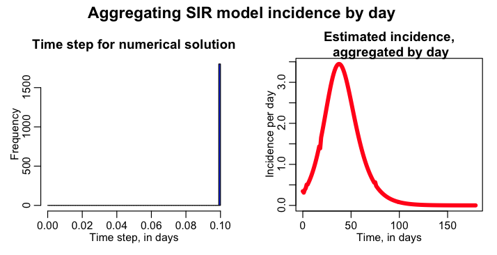
The added constraint on the size of delta_t has now largely eliminated the problem of choppiness in estimated daily incidence.
Questions:
- What would the estimated daily incidence look like if lconstrain_time_step=0, and we made N larger? How about N smaller?
- What would happen if I made k larger? smaller?
- Why, in the above histogram of the time step when lconstrain_time_step=1, is every single time step 0.1 days?
- How would we have to change the script if we wanted to aggregate by week, instead of day?
Another example: SEIR model
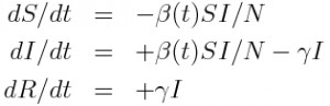
The ordinary differential equations for a Susceptible (S), Exposed (E), Infected (I), Recovered (R) compartmental model are:
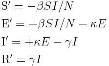
In this model, the flow of new individuals into the I compartment is kappa*E. That is to say, the change in incidence per unit time is kappa*E.
Question: if we are using a dynamical time step to numerically solve the model, what is the time step needed for, on average, one state transition to take place in the model?
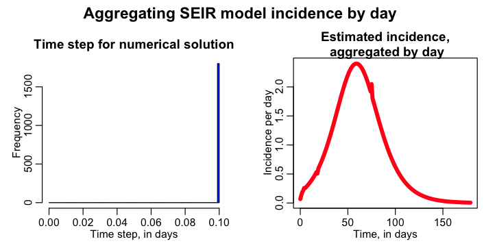
The R script seir_aggregate_incidence_by_day.R solves this model using a dynamical time step, under the hypothesis that R0=1.5, kappa=1/2, gamma=1/5, with initial conditions N=250, I=1, E=0, S=249, R=0. The script estimates the incidence per time step delta_t, and then aggregates by day, producing the following plot:
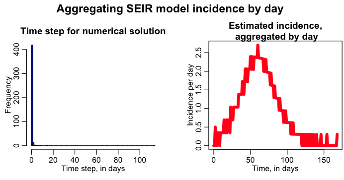
Again, just like with the SIR model with a dynamical time step solution, we have problems with choppiness when we try to aggregate the incidence by day.
The script has a logical variable lconstrain_time_step, that when equal to 1 ensures that the dynamical time step is, at most, 1/k days with k=10. Edit the seir_aggregate_incidence_by_day.R script to make this change and rerun it. It will produce the plot: