In this module students will become familiar with the Kolmogorov-Smirnov non-parametric test for equivalence of distributions

Sometimes in applied statistics we would like to test whether or not two sets of data appear to be drawn from the same underlying probability distribution.  Most of the time we don’t even know what that probability distribution is… it could be some crazily shaped distribution that doesn’t match a nicely behaved smooth distribution like the Normal distribution, for example.

As an example, read in the data file drug_mortality_and_2016_election_data.csv This file contains county-level data on per capita drug mortality rates from 2006 to 2016, along with the fraction of the voters in each county that voted Republican or Democrat in the 2016 presidential election.  Use the following code:

a = read.table("drug_mortality_and_2016_election_data.csv",header=T,as.is=T,sep=",")
a = subset(a,!is.na(rate_drug_death_2006_to_2016_wonder))

a_rep = subset(a,prep_2016>pdem_2016)
a_dem = subset(a,prep_2016<pdem_2016)

x1 = a_rep[,3]
x2 = a_dem[,3]
require("sfsmisc")
mult.fig(4)
breaks = seq(0,max(a$rate_drug_death_2006_to_2016_wonder),length=100)
hist(x1,col=2,main="Republican majority counties",xlab="Drug death rate",breaks=breaks,freq=F)
hist(x2,col=3,main="Democrat majority counties",xlab="Drug death rate",breaks=breaks,freq=F,add=F)

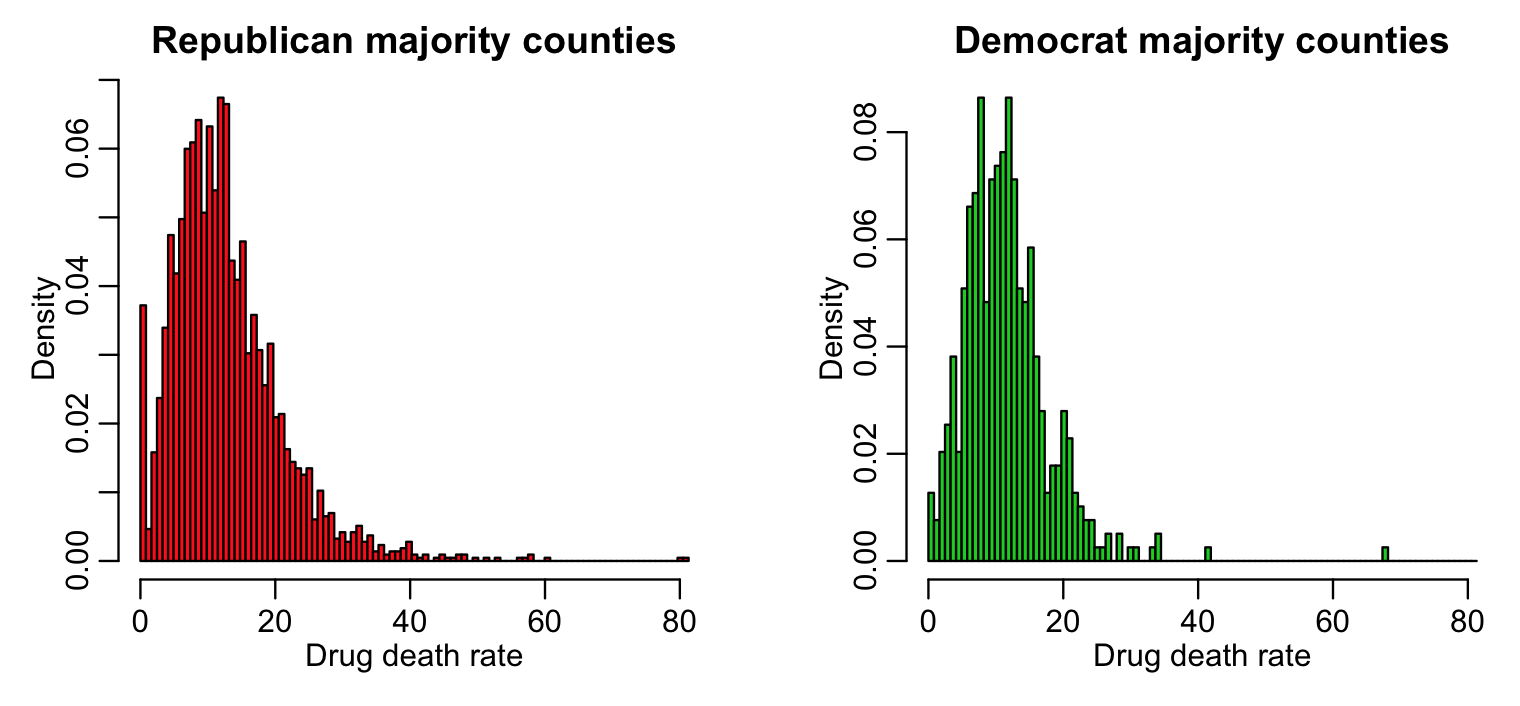
We would like to know if those two distributions are consistent with being drawn from the same underlying probability distribution.

To do this, we turn to what are known as non-parameteric tests.  “Non-parametric” means that we do not assume some parameterisation of the underlying probability distribution (for instance, by assuming it’s Normal).

The Kolmogorov-Smirnov test (KS test) is an example of one such test.  Given two data samples, X_1 and X_2, the algorithm first sorts both samples from smallest to largest, then creates a plot  that shows the cumulative fraction in each sample below each value of X (note that X_1 and X_2 data samples do not need to be the same size).  The KS test then looks at the maximum distance, D, between those two curves. As an example of this with our drug mortality data, use the code:

xtot = sort(c(x1,x2))
cumsum_x1 = numeric(0)
cumsum_x2 = numeric(0)
for (i in 1:length(xtot)){
 cumsum_x1 = c(cumsum_x1,sum(x1<xtot[i]))
 cumsum_x2 = c(cumsum_x2,sum(x2<xtot[i]))
}
cumsum_x1 = cumsum_x1/length(x1)
cumsum_x2 = cumsum_x2/length(x2)

mult.fig(1)
plot(xtot,cumsum_x1,type="l",col=2,lwd=8,ylab="Cumulative fraction in each sample",xlab="Drug death rate")
lines(xtot,cumsum_x2,col=3,lwd=8)
legend("bottomright",legend=c("Republican majority counties","Democrat majority counties"),col=c(2,3),lwd=4,bty="n")

D = abs(cumsum_x1-cumsum_x2)
iind = which.max(D)
arrows(xtot[iind],cumsum_x1[iind],xtot[iind],cumsum_x2[iind],code=3,lwd=4,length=0.1)

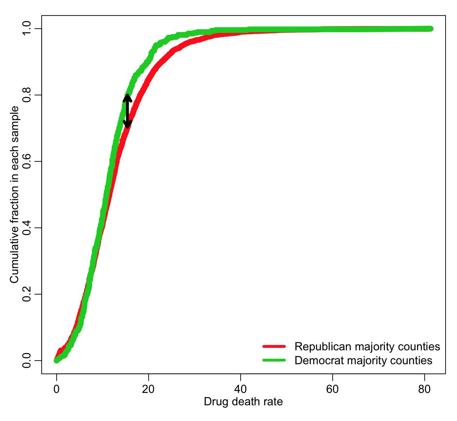
The larger the value of D, the greater the difference between the two distributions. The KS-test bases its statistical test on the value of D.

The KS-test is implemented in R with the ks.test() function.  It takes as its arguments the two samples of data.

k = ks.test(x1,x2)
print(k)

It prints out the p-value testing the null hypothesis that the two samples are drawn from the same distribution.

Difference between the KS test and the Students t-test

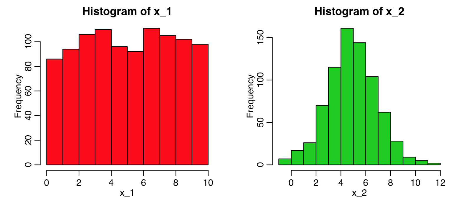
You may be wondering why we can’t just use a two sample Students t-test to determine if the means of the two distributions are statistically consistent.  You could of course do that, but two distributions can have dramatically different shapes, but have the same mean.

Here’s an example using simulated data where the two sample t-test shows the means of the samples are statistically consistent, but the KS test reveals they have very different shapes:

set.seed(8119990)
x_1 = runif(1000,0,10)
x_2 = rnorm(750,5,2)

require("sfsmisc")
mult.fig(4)
hist(x_1,col=2)
hist(x_2,col=3)

k = ks.test(x_1,x_2)
t = t.test(x_1,x_2)
print(k)
print(t)

KS test with a known probability distribution

The KS test can also be used parametrically, comparing the distribution of data to a known probability distribution.  For example, if we wanted to compare the x_1 distribution from the above example to a Uniform probability distribution between 0 and 1, we would type

k=ks.test(x_1,"punif",0,1)
print(k)

If we wanted to compare it to a Uniform probability distribution between 0 and 10:

k=ks.test(x_1,"punif",0,10)
print(k)

If we wanted to compare it to a Normal distribution with mean 5 and standard deviation 2:

k=ks.test(x_1,"pnorm",5,2)
print(k)

If we wanted to compare it to a Poisson distribution with mean 6:

k=ks.test(x_1,"ppois",6)
print(k)

You get the idea… just use the cumulative distribution function of the probability distribution you want to examine, along with the arguments for that probability distribution.