
In this module, students will become familiar with Negative Binomial likelihood fits for over-dispersed count data.
The Wikipedia pages for almost all probability distributions are excellent and very comprehensive (see, for instance, the page on the Normal distribution). The Negative Binomial distribution is one of the few distributions that (for application to epidemic/biological system modelling), I do not recommend reading the associated Wikipedia page. Instead, one of the best sources of information on the applicability of this distribution to epidemiology/population biology is this PLoS paper on the subject: Maximum Likelihood Estimation of the Negative Binomial Dispersion Parameter for Highly Overdispersed Data, with Applications to Infectious Diseases.
As the paper discusses, the Negative Binomial distribution is the distribution that underlies the stochasticity in over-dispersed count data. Over-dispersed count data means that the data have a greater degree of stochasticity than what one would expect from the Poisson distribution. In practice, this is frequently the case for count data arising in epidemic or population dynamics due to randomness in population movements or contact rates, and/or deficiencies in the model in capturing all intricacies of the population dynamics.
Recall that for count data with underlying stochasticity described by the Poisson distribution that the mean is mu=lambda, and the variance is sigma^2=lambda. In the case of the Negative Binomial distribution, the mean and variance are expressed in terms of two parameters, mu and alpha (note that in the PLoS paper above, m=mu, and k=1/alpha); the mean of the Negative Binomial distribution is mu=mu, and the variance is sigma^2=mu+alpha*mu^2. Notice that when alpha>0, the variance of the Negative Binomial distribution is always greater than the variance of the Poisson distribution.
There are several other formulations of the Negative Binomial distribution, but this is the one I’ve always seen used so far in analyses of biological and epidemic count data.
The probability of observing X counts with the Negative binomial distribution is (with m=mu and k=1/alpha):
![]() eqn 1
eqn 1
Recall that m is the model prediction, and depends on the model parameters.
Example comparison of Poisson distributed and over-dispersed Negative Binomially distributed data
The R function for random generation for the Negative Binomial distribution is in the same nightmare format as the Negative Binomial distribution as described on the Wikipedia page I told you not to read above because it’s pretty much incomprehensible. In the AML_course_libs.R file, I have thus put a function for you called my_rnbinom(n,m,alpha) that generates n Negative Binomially distributed random numbers with mean=m and dispersion parameter alpha.
Let’s use this function to generate some Negative Binomially distributed simulated data about some true model, and compare it to Poisson distributed data about the same model:
source("AML_course_libs.R")
##########################################
# true model for log of y is linear in x
##########################################
a = 4.00
b = 0.01
x = seq(0,100,0.01)
logy = a+b*x
ypred = exp(logy)
##########################################
# randomly generate Poisson distributed
# and Negative Binomially distributed
# simulated data about the true model
##########################################
set.seed(314300)
yobs = rpois(length(ypred),ypred)
alpha = 0.2
yobs_nb = my_rnbinom(length(ypred),ypred,alpha)
##########################################
# plot the data
##########################################
mult.fig(1)
ylim = c(min(c(yobs,yobs_nb)),max(c(yobs,yobs_nb)))
plot(x,yobs,cex=1.0,xlab="x",ylab="y",ylim=ylim)
points(x,yobs_nb,cex=1.2,col=2)
points(x,yobs,cex=1.0)
lines(x,ypred,col=3,lwd=5)
legend("topleft",legend=c("Poisson distributed data","Negative Binomial distributed data","True model"),col=c(1,2,3),lwd=5,cex=0.9,bty="n")
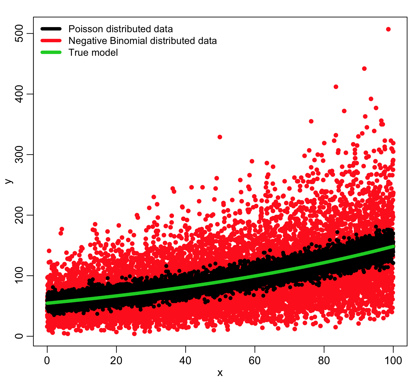
You can see that the Negative Binomially distributed data is much more broadly dispersed about the true model compared to the Poisson distributed data. The NB data are “over-dispersed”. In true life, nearly all count data are over-dispersed because of various confounders that may result in extra variation in the data over and above the hypothesized model (many of which are often unknowable).
Likelihood fitting with the Negative Binomial distribution
If we had N data points, we would take the product of the probabilities in Eqn 1 to get the overall likelihood for the model, and the best-fit parameters maximize this statistic. And just like we discussed with the Poisson likelihood, the negative of the sum of the logs of the individual probabilities (the negative log likelihood) is the statistic that is usually used, and minimized to determine the best-fit model parameters.
Just like the Poisson likelihood fit, the Negative Binomial likelihood fit uses a log-link for the model prediction, m.
In practice, using a Negative Binomial likelihood fit in place of a Poisson likelihood fit with count data will result in more or less the same central estimates of the fit parameters, but the confidence intervals on the fit estimates will be larger, because it has now been taken into account the fact that the data are more dispersed (have greater stochasticity) than the Poisson model allows for.
Let’s fit to our simulated data above, to illustrate this. The “MASS” package in R has a method called glm.nb that allows you to do Negative Binomial likelihood fits. If you don’t already have it installed, install it now by typing
install.packages(“MASS”)
Now let’s generate some simulated data that is truly over-dispersed, but fit it with Poisson likelihood then Negative Binomial likelihood:
a = 4.00
b = 0.001
x = seq(0,100,1)
logy = a+b*x
ypred = exp(logy)

set.seed(214388)
alpha = 0.2
yobs_overdispersed = my_rnbinom(length(ypred),ypred,alpha)

require("MASS")
pois_fit = glm(yobs_overdispersed~x,family="poisson")
NB_fit = glm.nb(yobs_overdispersed~x,control=glm.control(maxit=1000))

print(summary(pois_fit))
print(summary(NB_fit))
This produces the following results for the Poisson likelihood fit:

and these results for the NB likelihood fit:
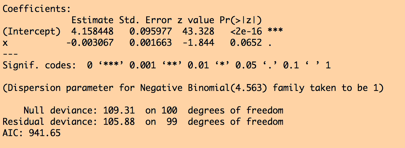
You can see that in the Poisson likelihood fit, the fit coefficient for x appears to be highly statistically significant. But in the Negative Binomial likelihood fit, the confidence intervals are much wider, and the x is no longer statistically significant… the NB likelihood fit properly takes into account the extreme over-dispersion in the data, and it properly adjusts the confidence intervals.
Of course, in our true model, log(y) really does depend on x, but if the data are very overdispersed, and/or you only have a few data points, it reduces sensitivity to be able to detect that relationship.
Moral of this story…
Virtually all count data you will encounter in real life are over-dispersed. In general, Negative Binomial likelihood fits are far more trustworthy to use with count data than Poisson likelihood… the confidence intervals on the fit coefficients will be correct. If you try both types of fits, and the p-values are more or less the same, you can default to the simpler Poisson fits.
But never use Poisson fit because you “like the answer better” that comes out of that fit compared to the NB fit (ie; the Poisson fit gives the apparently significant result you were “hoping” for, whereas it isn’t significant in the NB fit).
Model selection in R when using glm.nb()
Just like we saw with Least Squares fitting using the R lm() method, and Poisson and Binomial likelihood fits using the R glm() method, you can do model selection in multivariate fits with R glm.nb model objects using the R stepAIC() function in the “MASS” library.