[In this model, students will learn about some special properties of the Poisson, Exponential, and Gamma distributions.]

Exponential Distribution

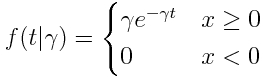
In compartmental modelling, the Exponential distribution plays a role as the probability distribution underlying the sojourn time in a compartment. As we discussed in this module, the Exponential distribution is continuous, defined on x=[0,infinity], with one parameter, gamma (also sometimes denoted with lambda, or rho, or some other letter)

T

he mean of the distribution is 1/gamma, and the variance is 1/gamma^2 The exponential distribution is the probability distribution for the expected waiting time between events, when the average wait time is 1/gamma.

Poisson Distribution

The Poisson distribution is discrete, defined in integers x=[0,inf].  It has one parameter, the mean lambda (or sometimes denoted gamma, or some other letter). With the Poisson distribution, the probability of observing k events when lambda are expected is: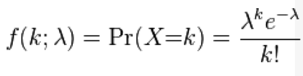
 
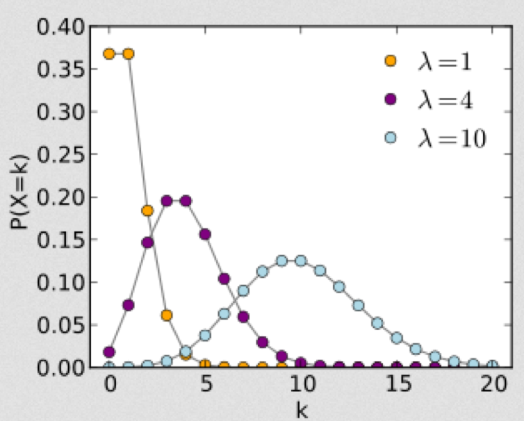Note that as lambda gets large, the distribution becomes more and more symmetric.  In fact, as lambda gets large (greater than around 10 or so), the Poisson distribution approaches the Normal distribution with mean=lambda, and variance=lambda.

Relationship between Exponential and Poisson distribution

There is an interesting, and key, relationship between the Poisson and Exponential distribution.  If you expect gamma events on average for each unit of time, then the average waiting time between events is Exponentially distributed, with parameter gamma (thus average wait time is 1/gamma), and the number of events counted in each unit of time is Poisson distributed with parameter gamma.

The Exponential distribution also describes the time between events in a Poisson process.  For instance, assume that gamma babies are on average born in a hospital each day, with underlying stochasticity described by the Poisson distribution.  It can be shown that the probability distribution for the wait time (in days) between babies is gamma*exp(-t*gamma)

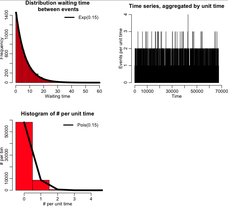
As another example, let’s examine the following R code that randomly generates 10000 distributed random variables, X, from the Exp(gamma=0.15) distribution.  If we interpret X as the waiting time from event to event (measured in days, for instance), this means the average waiting time is 1/gamma=6.7 days. The time that each event happens can be obtained from the cumulative sum of the waiting times from event to event.  We can then aggregate the number of events that happen per unit time, and histogram it.  The number of events per bin should be Poisson distributed as Pois(gamma). 

The following code, more heavily commented, is in the script exp_and_pois.R

require("sfsmisc")
set.seed(935662)
n = 10000
gamma = 0.15
cat("gamma is ",gamma,"\n")
mult.fig(4)
X = rexp(n,gamma)
cat("Average wait time is ",mean(X),"\n")
x = seq(0,60)
hist(X,breaks=seq(0,60),col=2,main="Distribution waiting time\n between events",xlab="Waiting time")
lines(x,dexp(x,gamma)*n,col=1,lwd=5)
legend("topright",legend=paste("Exp(",gamma,")",sep=""),lwd=3,bty="n")
##############################################################
# time that each event occurs is cumulative sum of wait times
##############################################################
vtime = cumsum(X)
##############################################################
# aggregate how many occur in each integer unit of time
##############################################################
g = hist(vtime,seq(0,max(as.integer(vtime)+1)),main="",xlab="Time",ylab="Events per unit time")
cat("Average number that occur each unit of time = ",mean(g$counts),"\n")
h=hist(g$counts,col=2,breaks=seq(-0.5,4.5),main="Histogram of \043 per unit time",xlab="\043 per unit time",ylab="\043 per bin")
x = seq(0,10)
lines(x,dpois(x,gamma)*sum(h$counts),col=1,lwd=5)
legend("topright",legend=paste("Pois(",gamma,")",sep=""),lwd=3,bty="n")

The script produces this plot, which shows the distribution of waiting times, the time series of the number of events per unit time, and the distribution of the number of events per unit time:

Gamma Distribution

The Gamma distribution is continuous, defined on t=[0,inf], and has two parameters called the scale factor, theta, and the shape factor, k.

The mean of the Gamma distribution is mu=k*theta, and the variance is sigma^2=k*theta^2.

When the shape parameter is an integer, the distribution is often referred to as the Erlang distribution.

The PDF of the Gamma distribution is

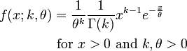For various values of k and theta the probability distribution looks like this:

Notice that when k=1, the Gamma distribution is the same as the Exponential distribution with lambda=1/theta.

When k>1, the most probable value of time (“x” in the function above) is no longer 0.  This is what makes the Gamma distribution much more appropriate to describe the probability distribution for time spent in a  state.

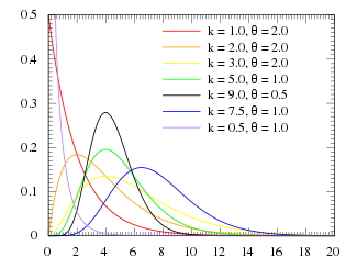
The sum of Exponentially distributed random numbers is Gamma distributed

If you have k Exponentially distributed random numbers, distributed according to Exp(lambda), X_1,…,X_k, their sum is distributed as Gamma(shape=k,scale=1/lambda).  Recall that the mean of the Gamma distribution is mu=shape*scale, and the variance is var=shape*scale^2. Try the following in R:

 require("sfsmisc")
 set.seed(935662)
 n = 10000
 gamma = 0.75
 X1 = rexp(n,gamma)
 X2 = rexp(n,gamma)
 X3 = rexp(n,gamma)
 k = 3
 Xsum = X1+X2+X3
 x = seq(0.5,19.5)
 aname = paste("Exp(",gamma,")",sep="")
 bname = paste("Gamma(",k,",",gamma,")",sep="")
 mult.fig(4)
 hist(X1,breaks=seq(0,20),col=2)
 lines(x,dexp(x,gamma)*10000,col=1,lwd=5)
 legend("topright",legend=aname,col=1,lwd=5,bty="n")
 hist(X2,breaks=seq(0,20),col=2)
 lines(x,dexp(x,gamma)*10000,col=1,lwd=5)
 legend("topright",legend=aname,col=1,lwd=5,bty="n")
 hist(X3,breaks=seq(0,20),col=2)
 lines(x,dexp(x,gamma)*10000,col=1,lwd=5)
 legend("topright",legend=aname,col=1,lwd=5,bty="n")
 hist(Xsum,breaks=seq(0,20),col=2,main="Histogram of Xsum=X1+X2+X3")
 lines(x,dgamma(x,shape=k,scale=1/gamma)*10000,col=1,lwd=5)
 legend("topright",legend=bname,col=1,lwd=5,bty="n")

This produces the following plot, that shows the histogram of X1, X2, X3 and their sum, when X1, X2, and X3 are Exponentially randomly distributed with gamma=0.75.  Their sum is thus Gamma distributed as Gamma(3,1/0.75)

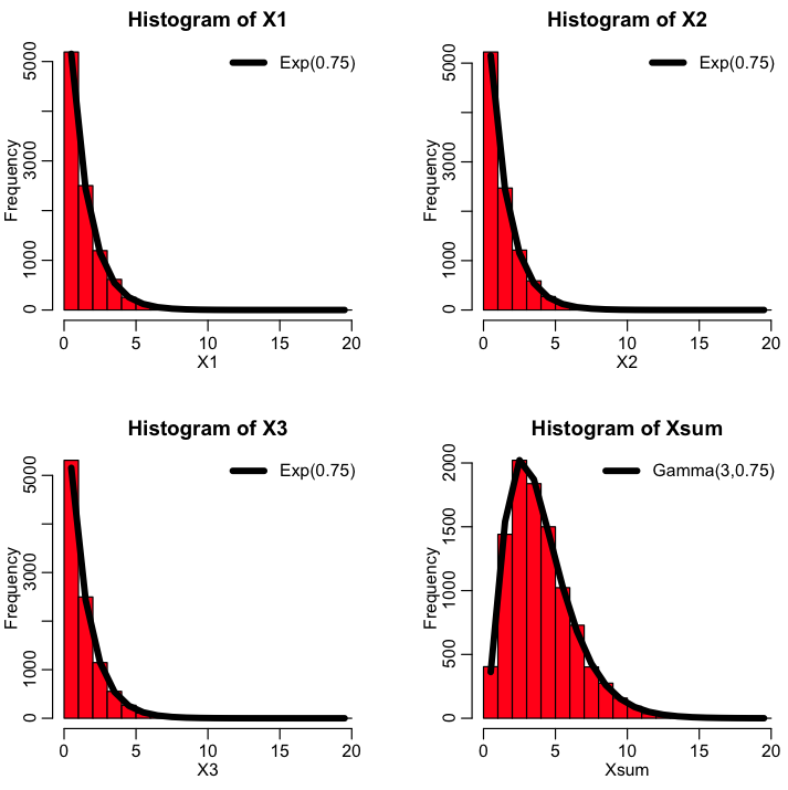
Interesting property of the Exponential distribution: If X~Exp(gamma) and Y~Exp(rho), then min(X,Y) is distributed as Exp(lambda) with lambda=gamma+rho

The proof of this property can be found here. (original source) As an example, let’s examine the following R code (also in the script minimum_two_exponentials.R):

require("sfsmisc")
set.seed(935662)

n = 10000
gamma = 0.35
rho = 0.65

######################################################
# get n randomly distributed numbers each according
# to Exp(gamma) and Exp(rho)
######################################################
X = rexp(n,gamma)
Y = rexp(n,rho)

######################################################
# now take, element by element, the minimum
# of X and Y. The R function pmin() does this
# pairwise minimum operation
######################################################
Z = pmin(X,Y) 

amax = max(as.integer(c(X,Y,Z)))+1
x = seq(0,amax)

mult.fig(4)
hist(X,breaks=seq(0,amax),col=2,main="Distribution X~Exp(gamma)",xlab="Waiting time")
lines(x,dexp(x,gamma)*n,col=1,lwd=5)
legend("topright",legend=paste("Exp(",gamma,")",sep=""),lwd=3,bty="n")

hist(Y,breaks=seq(0,amax),col=2,main="Distribution Y~Exp(rho)",xlab="Waiting time")
lines(x,dexp(x,rho)*n,col=1,lwd=5)
legend("topright",legend=paste("Exp(",rho,")",sep=""),lwd=3,bty="n")

lambda = gamma+rho
hist(Z,breaks=seq(0,amax),col=2,main="Distribution min(X,Y)",xlab="Waiting time")
lines(x,dexp(x,lambda)*n,col=1,lwd=5)
legend("topright",legend=paste("Exp(",lambda,")",sep=""),lwd=3,bty="n")

Note that I just happened to pick a gamma and rho that added to 1.  I could have picked any values. If we had X~Exp(gamma), Y~Exp(rho), and W~Exp(omega), and took Z~min(X,Y,Z), how do you think Z would be distributed?

Sum of two independent Poisson distributed random numbers is also Poisson distributed

If we have two independent random numbers, X~Pois(gamma), and Y~Pois(rho), then Z=X+Y is distributed as ~Pois(lambda=gamma+rho) The proof of this property can be found here. As an example take a look at the following R code (which is also in the R script sum_two_poisson.R):

require("sfsmisc")
set.seed(935662)

n = 10000
gamma = 2.7
rho = 1.5

######################################################
# get n randomly distributed numbers each according
# to Pois(gamma) and Pois(rho)
######################################################
X = rpois(n,gamma)
Y = rpois(n,rho)

######################################################
# now add them
######################################################
Z = X+Y

amax = max(Z)+1
xb = seq(-0.5,amax-0.5)
x = seq(0,amax)

mult.fig(4)
hist(X,breaks=xb,col=2,main="Distribution X~Pois(gamma)",xlab="X")
lines(x,dpois(x,gamma)*n,col=1,lwd=5)
legend("topright",legend=paste("Pois(",gamma,")",sep=""),lwd=3,bty="n")

hist(Y,breaks=xb,col=2,main="Distribution Y~Pois(rho)",xlab="Y")
lines(x,dpois(x,rho)*n,col=1,lwd=5)
legend("topright",legend=paste("Pois(",rho,")",sep=""),lwd=3,bty="n")

lambda = gamma+rho
hist(Z,breaks=xb,col=2,main="Distribution X+Y",xlab="Z=X+Y")
lines(x,dpois(x,lambda)*n,col=1,lwd=5)
legend("topright",legend=paste("Pois(",lambda,")",sep=""),lwd=3,bty="n")

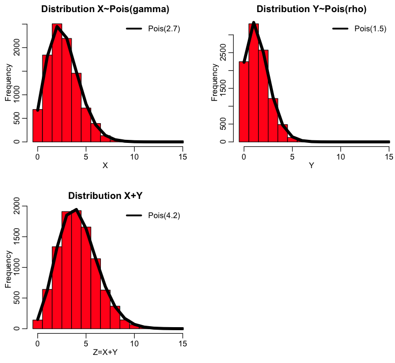
If we have three random variables drawn from X~Pois(gamma), Y~Pois(rho), W~Pois(omega), how do you think their sum Z=X+Y+W is distributed?

Sum of two Normally distributed random numbers is also Normally distributed

While we’re on the topic on the distribution of the sum Poisson random numbers, it is worth briefly mentioning that the sum of two Normally distributed random variables is also a Normally distributed random variable. Thus, if X~Norm(mu1,sigma1) and Y~Norm(mu2,sigma2), then Z= X+Y is distributed as Z~Norm(mu3,sigma3), with mu3=(mu1+mu2) and sigma3=sqrt(sigma1^2+sigma2^2).

“Memoryless” property of the Exponential distribution

An interesting, and important, property of the Exponential distribution is that the probability of an individual leaving a compartment in a small time step is completely independent of the time the individual has spent in the compartment when the sojourn time in the compartment is Exponentially distributed.

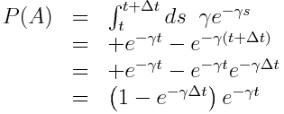
To show why this is the case, let’s calculate the probability that, for instance, an infected individual in an SIR model will recover between times t to t+delta_t (refer to this as event “A”), given that the individual has been infected up until time t (refer to this as event “B”), and the rate for leaving the compartment is gamma (recall that compartmental models inherently assume the probability distribution for the sojourn time in the compartment is Exponentially distributed).  Baye’s theorem tells us that

P(A|B) = P(B|A)P(A)/P(B)

“P(A|B)” is read as “the probability that A occurs, given that B occurs”.

“P(A)” is read as “the probability that A occurs”.

It’s easy to see that P(B|A)=1 because A occurring necessarily implies that B must have occurred too; in order to recover between times t and t+delta_t (A), it has to be true that the individual was still in the infectious compartment at time t (B).

The exponential probability distribution underlying the sojourn time in the infectious compartment is f(t) = gamma exp(-gamma*t), where gamma is the average recovery rate. We can easily calculate, by integrating the probability distribution, that

and

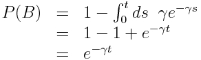
Thus, with

P(A) = (1-exp(-gamma*delta_t))*exp(-gamma*t), 
and 
P(B) = exp(-gamma*t).

and

P(A|B) = P(A)/P(B)

we get

P(A|B) = 1-exp(-gamma*delta_t)

Notice that this does not depend on time!  The probability of leaving the infectious state is constant in time, and does not depend on how long an individual has been infectious.  This is know as the “memoryless” property of the exponential distribution.

When delta_t is small, 1-exp(-gamma*delta_t)~gamma*delta_t

Note that if we Taylor expand P=1-exp(-gamma*delta_t) around 0, we find that, to first order, P~gamma*delta_t.   You will recognize this as the expected number of changes of state in time delta_t in a compartmental model with just one individual in the compartment, and rate of leaving the compartment equal to gamma.

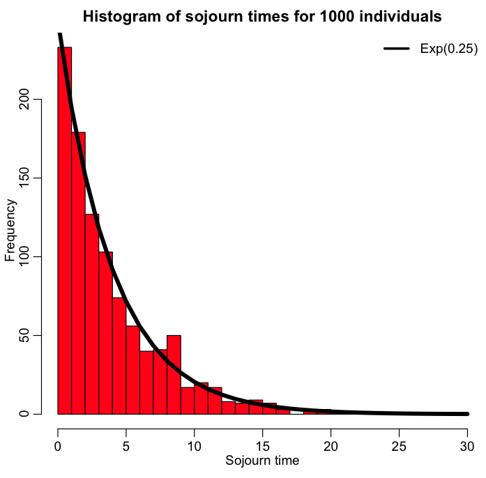
Simulating the time an individual spends in a state, when the expected sojourn time is Exponentially distributed

In practical terms, how would we, in an Agent Based model for instance, simulate the time an individual spends in a state, when the expected sojourn time is Exponentially distributed? As we saw above, the Exponential distribution is memoryless, and the probability of leaving a state between time t and t+delta_t is constant, and equal to

P=1-exp(-gamma*delta_t),

when the parameter of the Exponential distribution is gamma. Thus, as we step through time in small time steps, we

1. Randomly sample a number from the Uniform distribution between 0 and 1.
2. If that number is less than P, the individual leaves the state.  If the number is greater than P, then the individual remains in the state, and we move on to the next time step.

Repeat steps 1 and 2 until the individual leaves the state.  Because the Exponential distribution is memoryless, we don’t need to keep track of how long an individual has been in the state to calculate the probability that it will leave it. This way of simulating sojourn times in a state is useful for both Markov Chain Monte Carlo, and Agent Based modelling.

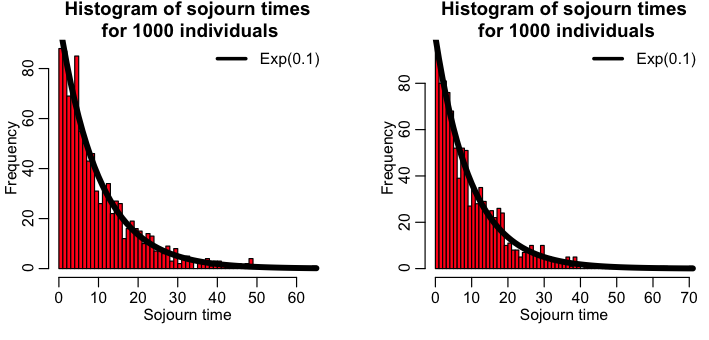
The R script simulate_individual_leave_state_exponential.R performs this process for 1000 individuals in a state where the rate of leaving the state is gamma=1/4.  The script produces the plot:

However, there is more than one way to skin the Exponential stochastic cat.   In the R script simulate_individual_leave_state_exponential_b.R, I show how we can simulate this simple system of one compartment two other different ways, including sampling the Exponential distribution to determine the time between state transitions, and also directly sampling the Exponential distribution.  The script produces the plot:

Simulating the time an individual spends in a state, when the expected sojourn time is Gamma distributed

In the above we examined how we would simulate the sojourn time when the underlying probability distribution is Exponentially distributed.  The fact that the Exponential distribution is memoryless simplifies that simulation process considerably, because we don’t have to keep track of how long an individual has been in a state, because the probability of leaving the state in a set time step is constant. But Exponential probability distributions for state sojourn times are usually unrealistic, because with the Exponential distribution the most probable time to leave the state is at t=0.

Recall that the Erlang distribution is the distribution of the sum of k independent Exponentially distributed random variables with mean theta.  It turns out that this property provides a convenient means to incorporate an Erlang distributed probability distribution for the sojourn time  into a compartmental model in a straightforward fashion; for instance, assume that the sojourn time in the infectious stage of an SIR model is Erlang distributed with k=2 and theta = 1.5 (with 1/gamma = k*theta)… simply make k infectious compartments, each of which (but the last) flows into the next with rate gamma*k.  The last compartment flows into the recovered compartment:

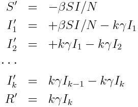
So, to simulate a Gamma (Erlang) distributed sojourn time in a stochastic simulation of a compartmental model, we expand the model with multiple compartments as above, and carry on as we normally would in our stochastic simulation methods.