
In this module, students will learn how the Least Squares fit statistic can be expressed as a likelihood.
Previous modules have discussed regression using the Least Squares fit statistic, and also Poisson and Binomial (logistic) likelihood fits.
Likelihood fits can sometimes seem a bit daunting to first time users, because Least Squares is a very intuitive fit statistic (minimizing the sum of squares of the distances between the data points and the model), but likelihoods perhaps less so. It perhaps doesn’t help that it is usually not pointed out that Least Squares itself is a fit statistic derived from a likelihood expression, and minimizing the Least Squares statistic maximizes that likelihood.
Recall that the underlying assumptions of the Least Squares fitting method are that the data are Normally distributed, with the same standard deviation, sigma (ie; the data are homoskedastic), and the points are independently distributed about the true model, mu.
This means that the probability distribution for some observed dependent variable, y, is the Normal distribution:
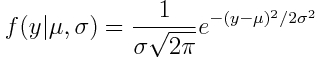 eqn 1
eqn 1
Note that mu might depend on some explanatory variables. Perhaps in a linear fashion, like (for example)
![]()
Now, just like we saw in the modules on Poisson and Binomial regression, the Least Squares likelihood of observing some set of dependent variables, y_i, given predicted model values for each point, mu_i, is derived from the product of the probability densities seen in Equation 1
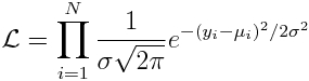 Eqn 2
Eqn 2
(note that the sigma is the same for each data point because of the homoskedasticity assumption of Least Squares). The best fit parameters in the mu_i function will maximize this likelihood. You could call this likelihood the “homoskedastic Normal likelihood”.
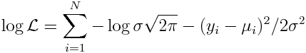
Recall that having a product of probabilities (all of which are between 0 and 1) can be problematic in practical computation because of underflow errors when using numerical methods to optimize the likelihood. Thus, in practice, we always take the log of both sides of the likelihood equation (the parameters in the calculation of mu that maximize the likelihood will also maximize the log likelihood).
This yields:
As we discussed in the Poisson and Binomial regression modules, in practice, numerical optimization methods in the underlying guts of statistical software packages minimize goodness-of-fit statistics, rather than maximize them. For this reason, we minimize the negative log likelihood:
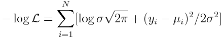
Notice that because sigma is the same for all points, the first term is just a constant. And you’ll recognize the second term as the Least Squares statistic divided by 2*sigma^2.
Thus, whatever model parameters that go into the calculation of mu_i that minimize the Least Squares statistic will also minimize the Normal negative log likelihood!
And thus Least Squares fits can equivalently be thought of as a homoskedastic Normal likelihood fit.