[This post is part of a series of posts on archaeoastronomy using open source software]

After you have obtained a satellite image of an archaeological site, uploaded the image to the XFig graphical software package, and placed datum points on site features, you can get XFig to output the datum point coordinate information into a text file in Computer Graphics Metafile (CGM) format.

You can then use the free and open-source R statistical programming language to read in the CGM files and fit straight lines between the datum points. R is not only a programming language, but also has graphics and a very large suite of statistical tools. Connecting models to data is a process that requires statistical tools, and R provides those tools, plus a lot more.

If you need an introduction to the R programming language, I’ve written posts on the topic.

The files that I obtained in my datum-point laying process described above are in the tarred directory merry_maidens.tar.gz  You will need to download these files to your working directory to run the R code below.

The R program merry_maidens_read_cgm.R reads in all the cgm files and calculates the average positions and radii (in real world coordinates) of the 21 datum points.  You will notice that I’ve made the file easy to modify to use your own place name, your own number of datum-point files, and the scale shown on your satellite image.  The program outputs the summarized data in the text file merry_maidens_avg_datum_points.txt which will be read into subsequent programs that fit lines between the points.

The R script merry_maidens_overlay.R reads in the GIF figure of the Google R screen shot (in the file merry_maidens.gif), and overlays the average datum points from the file above on the figure. This script requires that you have downloaded the caTools and sfsmisc libraries. You will also need the file with helper functions I’ve written (in this case, a function that draws circles) in the file archeoastronomy_libs.R. The merry_maidens_overlay.R script produces the following image: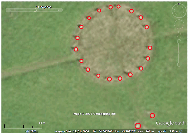

(Note that I have made the script easy to modify to include your own site name.)

The script is easy to modify this file to overlay lines connecting the datum points, but first we need to fit those lines. Note that the size of the stones is non-negligible compared to the distance between the stones.  In addition, the stones are low enough that they could either be used as sight lines across the centers of the stones (but this seems improbable as a precise sighting method, given how broad the stones are), or sight lines along the edges of the stones (if you are sitting near the ground).  Or perhaps you could be standing with your back to one of the stones and looking tangent to one or more stones.

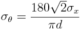
But first we must take into account the consideration that some of the stones are too close together to act as precise sight lines to the horizon.  How far apart do the datum points need to be?  If we connect just two points, and we call the uncertainty on the x and y position of the points sigma_x, and sigma_y, respectively, and assume they are roughly equal, then the formula for the uncertainty, in degrees, on the angle between two points a distance d apart is approximately

 Eqn(1)

I usually take a conservative approach, and assume that sigma_x is the maximum uncertainty on x or y in the points in my sample.  In the case of the Merry Maidens data, the maximum positional uncertainty calculated from the 10 datum point superimposition iterations is sigma_x~3.4 cm.  From Eqn(1) we see that to get an angular uncertainty of exactly one degree, the minimum distance between points can be calculated from

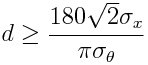 Eqn(2)

to be d>275cm (ie; at least 9 feet apart). In reality, we should aim for better precision than this, otherwise it becomes difficult to truly determine what direction the stone alignment is pointing. What precision you desire is up to you (and of course the reviewers of any of your published research) to decide, but something less than at most half of a degree precision for the angle connecting a set of points is probably good to aim for. Note that the more datum points along a line, generally the better the angular precision of the site line will be, as we’ll discuss in the next section.

 

 

Fitting lines to more than two points

A problem with fitting to just two points is that there is always a straight line that goes exactly through the centers of those two points.  You can thus end up with a lot of spurious site lines that have nothing to do with astronomical alignments.  It is thus more prudent to ascertain site lines by fitting to combination of three or more points, by minimizing some goodness-of-fit statistic.   Fitting to more points can also substantially decrease the uncertainty on the angle of the line that goes through them, if the points really are co-linear.

Let’s assume that our predicted line, with slope m and intercept b, is

where x_obs is our observed x positions of the points. If we assume that our uncertainty in x and y positions of the points are sigma_x and sigma_y, then the uncertainty on Y_pred is

If we have N points we are fitting to, we can obtain the best-fit line by minimizing the chi-squared statistic T

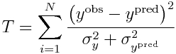
which is equal to

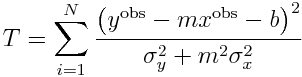 Eqn 3

Under the null hypothesis that the N points truly do lie in a straight line, the probability distribution for T will be chi-squared with N-2 degrees of freedom (assuming that you got your estimates of sigma_x and sigma_y right). People who have some experience with regression methods will recognize T as a weighted least squares statistic.

Obtaining the uncertainty on m and b involves taking the inverse of the Hessian matrix of Eqn 3, which can be tedious (if not downright impossible for you to do if you’ve never taken calculus!). Luckily, we can use the R optim() function to find the values of m and b that minimize Eqn 3, and also calculate the uncertainty on them.

The function mychisquared() in archeoastronomy_libs.R calculates the chi-squared statistic in Equation 3.  The function fit_line(x,y,sigmax,sigmay) in archeoastronomy_libs.R uses the mychisquared() function in conjunction with the R optim() function to find the slope of the line, and its uncertainty.  The fit_line(x,y,sigmax,sigmay) function translates this slope into an estimated rise/set azimuth (in degrees) that the line is pointing to, along with the uncertainty on that.  It takes as its arguments the vector of x, y, sigma_x and sigma_y points.  The function also returns the minimum value of the T statistic from Equation 3, and the adjusted R^2 statistic of the fit.

The find_all_possible_combos(N,k) returns in a matrix, matrix_of_indices, all possible unique combinations of indices of N data points, taken in groups of k at a time.  The rows of matrix_of_indices correspond to each unique combination, and the columns of matrix_of_indices are the indices of the data point. Note that the number of possible unique combinations is choose(N,k), so taking a large value of k will take a long time to calculate all the possible indices, and will return a *huge* matrix!

Deciding the criteria on what to consider a good fit is a bit tricky.  You can use the chi-squared null hypothesis test using the assumption that T is distributed as a chi-squared with N-2 degrees of freedom.  However, this assumes that you got your estimates of sigma_x and sigma_y exactly right.

The adjusted R^2 of the fit is probably a better choice.  To determine what the cutoff value for this should be in order to declare that a set of points apparently forms a straight line, I prefer to fit to randomly scrambled versions of the points in the site map, and then look at the distributions of the adjusted R^2 I get from those fits.  If I choose the cutoff in the adjusted R^2 such that only, for instance, 1% of those random fits return apparent straight line configurations of points, I know that in my true site map if I use that cutoff I can be 99% sure that the points aren’t aligning by mere random chance.

I try to take a conservative approach when I do this, and normally just don’t fit to random points scattered in a plane, but assume that there was some reason the ancient society placed the points in the approximate patterns that they did, and try to maintain those patterns as much as possible.

For instance, for the Merry Maidens site, I would assume that they spaced the stones in the circle exactly as they wanted them spaced in a circle of that radius, perhaps for aesthetic or ceremonial reasons that have nothing to do with astronomical alignments.  And I would assume that the distance of the outlier stones from the circle also is something the builders desired for some reason.

I then randomly change the placement of the two outlier stones around the circle, under the constraint that they remain the same distance away from the center of the circle.  Then I fit to all combos of three points and calculate the adjusted R^2. I do this many times, and thus get the distribution for the adjusted R^2 under the null hypothesis that placement of the outlier stones is random.