
[In this module, students will become familiar with Markov Chain Monte Carlo, and what processes can and cannot be modelled with MCMC. Simple examples of SIR and SEIR disease models will be presented.]
Markov Chains are a random process by which a system transitions from one state to another within a state space. They are memoryless, in the sense that the possible states the system can transition to at time t depend only on the current state of the system, not on how it got there.
Examples of processes that are NOT Markov Chains
Self-excitation in Mass Killings

An example of a process that is NOT a Markov Chain is a self-excitation process, where prior past events temporarily increase the probability that a similar event will occur in the immediate future.
An example of a system that can be modelled with a self-excitation process is mass killings; we can model mass killings by assuming that there is some baseline probability distribution for a mass killing to occur on any particular day, but when a mass killing occurs, it temporarily increases the probability, over and above the baseline probability, for a similar event to occur in the near future (ie; copycat events). Thus, the probability that a mass killing occurs on a certain day depends on the temporal distribution of all prior mass killings, and how far distant they were in the past. The system is NOT memoryless, and thus is NOT a Markov Chain Monte Carlo process.
Self-excitation in Earthquakes
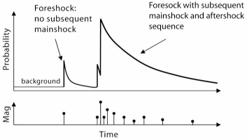
Another example is earthquakes; the probability that there will be an earthquake at a location depends a lot on when prior earthquakes have occurred there. The system is NOT memoryless, and thus is NOT a Markov Chain Monte Carlo process. Another example of a non-Markov process is drawing coins from a purse.
Examples of systems that CAN be modelled with Markov Chains
Predator/prey

An example of a system that can be modelled as a Markov Chain is a predator/prey system. If you have, on a particular day, 10 foxes and 100 rabbits, the number of rabbits and foxes are born in the next time step, and the number of rabbits that get eaten, doesn’t matter how you got to 10 foxes and 100 rabbits in that population. Maybe you just released those foxes and rabbits on that day into an empty forest. Or maybe both the rabbit and fox populations have been in decline for some time, and 10 years ago there were 100,000 foxes, and 100 million rabbits. What happened 10 years ago doesn’t matter when it comes to assessing what will happen in the next time step. It only matters how many each of foxes and rabbits there are at time t, and what the birth rates, predator and prey natural death rates, and predation rates are. As an aside, a population of 10 foxes and 100 rabbits is entirely appropriate to model with Markov Chain Monte Carlo. As we discussed in a previous module, a population with 100,000 foxes and 100 million rabbits is more appropriately modelled with an SDE, because modelling it with a Markov Chain Monte Carlo would be too computationally intensive.
Baseball

Another, classic, example of a Markov Chain process is a baseball game. If you, at time t, have no one on base and two out, there are only 5 possible outcomes at the next at-bat; person on first, person on second, person on third, home run, or out. The list of potential transition states do not depend on what happened prior in the game that led to the particular current state.
Markov Chain Monte Carlo Modelling
Coding up an MCMC stochastic compartmental model consists of the following steps
- Start with the compartments in some initial condition
- Determine all possible changes of +1 or -1 that can occur in the number of individuals in the compartments
- Based on the current state of the system, determine the time step, delta_t, needed for just one individual to change compartments in the entire system, on average
- Determine the average number of times, based on the current state of the system, that each of the possible transitions will take place in time delta_t
- Sample Poisson distributed random numbers based on these probabilities. Increment the compartments accordingly, and increment the time by +delta_t
- Repeat steps 2 to 5 for as many time steps as desired, or some condition is reached (for instance, no transitions are possible due to the state of the system…for example, in a closed predator/prey system, no transitions of +/1 individuals in the compartments are possible if all the predators and prey are dead).
Example: Susceptible, Infected, Recovered (SIR) Disease Model
As an example of the above steps, let’s look at a simple SIR disease model. Assume that we begin with a closed population of N individuals, one of whom is infected, and the rest of whom are susceptible. We thus have S=N-1, I=1, R=0 The set of ODE’s describing the dynamics of the system are:
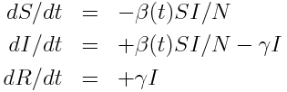 I
I
n this system, assuming I>0, we can have the transitions
- delta_S = -1, delta_I = +1 (infection)
- delta_I = -1, delta_R = +1 (recovery)
Note that if I=0, no transitions are possible, because there is no one left to recover, and no one left to infect the remaining susceptibles. The time step, delta_t, for on average just one transition in the system is
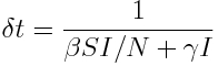
Tabulating the transition probabilities in that time delta_t yields
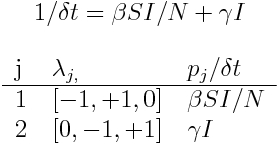
Now, if delta_t is the time needed for, on average, just one of the transitions to take place, the average number of times the first transition takes place in time delta_t is p_1=delta_t*beta*S*I/N, and the average number of times the second transition takes place in time delta_t is p_2=delta_t*gamma*I. Both numbers are less than 1. In simulating a Markov Chain Monte Carlo, to determine the number of transitions of type j in the next time step, when on average in that time step one transition of any kind will occur, we randomly Poisson sample a number from Pois(lambda=p_j). Because p_j is at most one for all j when we define delta_t this way, most often the Poisson random numbers will be around 0 or 1. Try in R, for instance,
hist(rpois(10000,0.1))
This should produce a plot similar to the following:
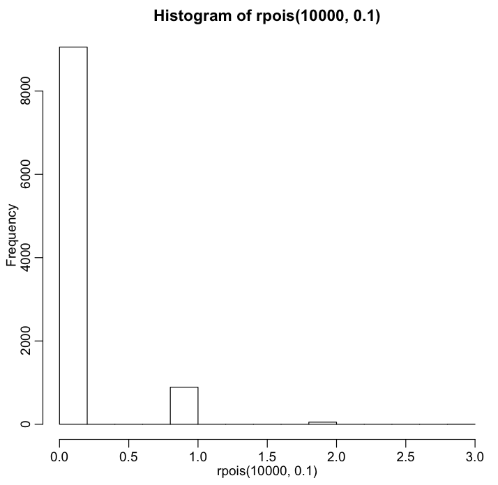 From the histogram, we see that if p_j=0.1, then most of the time sampling a Poisson distributed random number with lambda=0.1 will produce 0, sometimes 1, and very rarely 2 or more. Try making the histogram with p_j = 0.9. It is worth noting here that the sum of two Poisson random numbers drawn from Pois(lambda1) and Pois(lambda2) will itself be a Poisson random number distributed as Pois(lambda1+lambda2). You can try exploring this in R:
n = 10000
y1 = rpois(n,0.1)
y2 = rpois(n,0.7)
y3 = rpois(n,0.2)
y = y1+y2+y3
cat("The expected mean and sd of Pois(lambda( distribution are lambda and sqrt(lambda)\n")
cat("The observed mean and sd of the random numbers are",mean(y),sd(y),"\n")
Thus, when we define delta_t as we do above, and randomly sample Poisson random numbers from Pois(p_1), Pois(p_2),…..,Pois(p_J), the sum of those random numbers is distributed as Pois(1) because p_1+p_2+….+p_J=1. Which is exactly what we’d expect, because we’ve defined delta_t to be the time needed for, on average, one transition to take place.
So, let’s put this all together, and write an R script to do Markov Chain Monte Carlo modelling with this simple SIR model. The code is in the script sir_markov_chain.R
set.seed(156829)
gamma = 1/3 # recovery period in days^{-1}
R0 = 1.5 # R0 of R of the disease
beta = gamma*R0
N = 1000 # population size
I = 10 # number initially infected people in the population
S = N-I
R = 0
time = 0
vstate = c(S,I,R)
K = length(vstate) # number of compartments
J = 2 # number of possible state changes
# setup the matrix of state transitions...
lambda = matrix(0,nrow=J,ncol=length(vstate))
lambda[1,] = c(-1,1,0)
lambda[2,] = c(0,-1,1)
zstate = list()
i = 1 # iterator for the zstate list
while(vstate[2]>0&vstate[1]>0){
zstate[[i]] = c(vstate,time)
delta_t = 1/(beta*vstate[1]*vstate[2]/N + gamma*vstate[2])
l1 = rpois(1,(beta*vstate[1]*vstate[2]/N)*delta_t)
l2 = rpois(1,gamma*vstate[2]*delta_t)
vec_l = c(l1,l2)
vstate = vstate + vec_l%*%lambda
vstate[vstate<0] = 0
i = i+1
time = time + delta_t
if (i%%100==1) cat(i,time,vstate,"\n")
}
par(mfrow=c(2,2))
vS = sapply(zstate, "[[", 1)
vI = sapply(zstate, "[[", 2)
vR = sapply(zstate, "[[", 3)
vtime = sapply(zstate, "[[", 4)
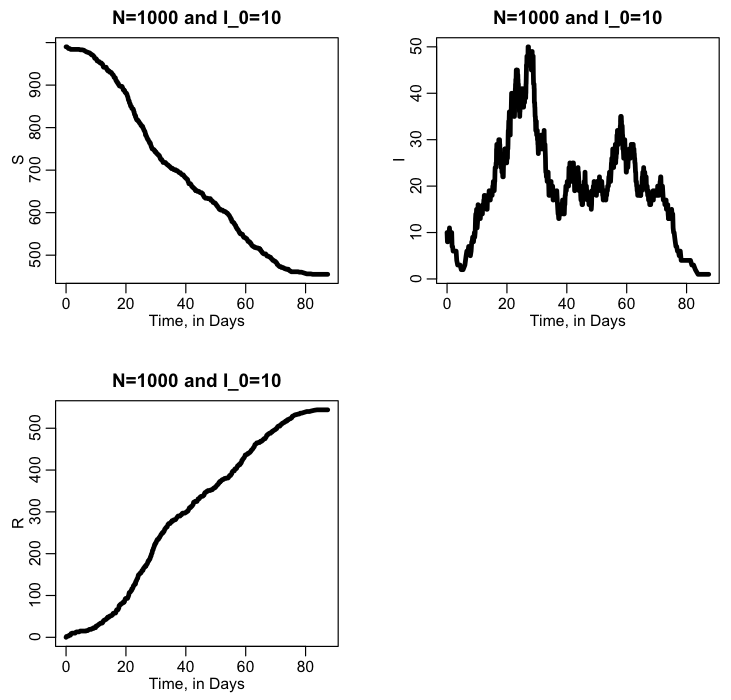
plot(vtime,vS,type="l",lwd=3,xlab="Time, in Days",ylab="S",main=paste("N=",N," and I_0=",vI[1],sep=""))
plot(vtime,vI,type="l",lwd=3,xlab="Time, in Days",ylab="I",main=paste("N=",N," and I_0=",vI[1],sep=""))
plot(vtime,vR,type="l",lwd=3,xlab="Time, in Days",ylab="R",main=paste("N=",N," and I_0=",vI[1],sep=""))
The script produces the following plot:
Questions:
- Why did I set the random seed at the beginning of the script?
- What will happen if I change the random seed?
- What assumptions does this model make?
- Are the assumptions realistic?
- What, in general, will happen to the prediction for the final size, epidemic curve, etc, if I change the value of gamma?
- What will happen if I change the value of R0?
- What will happen if I change the value of I_0, the initial number infected?
- What will happen if I change the population size, N?
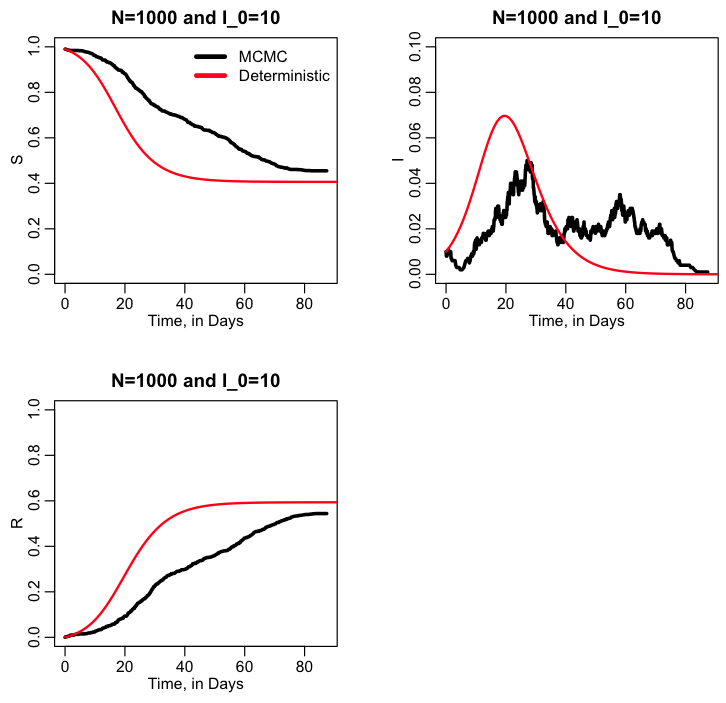
Adding in comparison to the deterministic model
It is always instructive to compare the stochastic model to the results of the deterministic model. The R script sir_markov_chain_compare_deterministic.R does this using methods from the R deSolve library to solve the ODE’s, and produces the following plot:
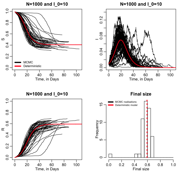
Why do stochastic modelling in the first place?
It is important to note in the exercise we just did that we did just one realisation of the stochastic model. When it comes to stochastic modelling, just one realisation is useless to infer anything. Which leads to the topic: why are we doing stochastic modelling in the first place? There are many reasons for stochastic modelling of dynamical systems. For instance, in the case of disease, you may be interested in the probability for an outbreak will occur given some initial conditions. And/or we might be interested in what the posterior probability distribution is for the final size (total number infected), peak incidence, or time of the peak, or how often the peak incidence exceeds some threshold (ie; because of hospital capacity issues, for instance). For populations, we may be interested in extinction probability after some time period, or the probability that a newly introduced species will maintain a viable population, or probability that the population will exceed some threshold. To assess these things, you have to run many realisations of the stochastic model and then histogram the results (or equivalently analyse them using other methodologies) to obtain “posterior probability distributions” for the quantity of interest. The R script sir_markov_chain_iterated.R performs 50 realisations of our SIR MCMC model, and then overlays all the results for S, I, and R into a summary plot, along with the results from the deterministic model. It also histograms the final size of the epidemic, and overlays a red dotted line showing the final size expected from the deterministic model:
 The R script also calculates the expected probability of an outbreak for an SIR or SIS disease model, given the initial number infected, I_0, and the reproduction number, R0: probability outbreak = 1-(1/R0)^I_0 (the derivation of this can be found in section 3.6.1 of Mathematical Epidemiology, edited by Brauer, van den Driessche, and Wu)
A slightly more complicated example: MCMC modelling of an SEIR model
The Susceptible, Exposed, Infected, Recovered model is described by the set of differential equations:
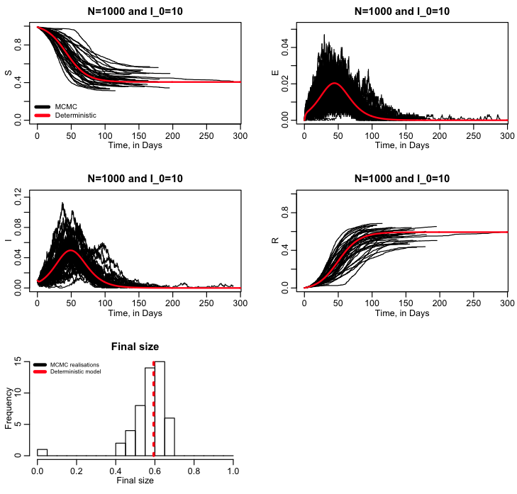
The R script seir_markov_chain_iterated.R performs 50 realisations of an SEIR MCMC model, and then overlays all the results for S, E, I, and R into a summary plot, along with the results from the deterministic model. It also histograms the final size of the epidemic, and overlays a red dotted line showing the final size expected from the deterministic model:
Could we have used a constant time step instead of a dynamical time step?
In all of the above examples, we used a dynamical time step to ensure that, on average, just one transition would take place each time step. Could we have used a constant time step instead?