[After reading through this module you should have an intuitive understanding of how infectious disease spreads in the population, and how that process can be described using a compartmental model with flow between the compartments.  You should be able to write down the differential equations of a simple disease model, and you will learn in this module how to numerically solve those differential equations in R to obtain the model estimate of the epidemic curve]

An excellent reference book with background material related to these lectures is Mathematical Epidemiology by Brauer et al. 

Contents:

• Introduction
• Basic dynamics of infectious disease spread
• The SIR compartmental model of disease spread
• The SIR model system of equations
• Numerically solving the SIR model system of equations in R
• R code to model an influenza pandemic with an SIR model
• Further things you can explore
• Summary

Introduction

Models of disease spread can yield insights into the mechanisms and dynamics most important to the spread of disease (especially when the models are compared to epidemic data).  With this improved understanding, more effective disease intervention strategies can potentially be developed. Sometimes disease models are also used to forecast the course of an epidemic, and doing exactly that for the 2009 pandemic was my introduction to the field of computational epidemiology.

There are lots of different ways to model epidemics, and there are several modules on this site on the topic, but let’s begin with one of the simplest epidemic models for an infectious disease like influenza: the Susceptible, Infected, Recovered (SIR) model.

Basic dynamics of infectious disease spread

With the SIR model, you start with a population of people who are susceptible to some infectious disease (say, influenza).  Initially a few infected people are added to the population and the entire population mixes homogeneously (meaning that the people an individual contacts each day are completely random).  During the duration of their illness the infectious people each infect on average X other people, who each then go on to and infect X other people, and so on, and so on, and so on.  Can you see that the number of infected people in the population will grow exponentially?  In fact, it can be shown that the exponential growth rate is equal to (X-1) divided by the length of the infectious period.

However, the exponential growth will eventually slow down, because the infected people recover and are now immune to the disease (in the SIR model, anyway… a model where they recover and then immediately become susceptible again is called a SIS model, and a model where people get infected and remain infected is an SI model); thus each infected person will still contact X other people during the course of their illness, but as time goes on a larger and larger fraction of the people they contact will be immune to the disease.  As this happens the spread of the disease slows, and eventually starts to decline.

X is a very special quantity.  Because it is the average number of people in a fully susceptible population that an infected person infects, it can be thought of as the number of infected people an infected person can reproduce.  In epidemiology, we thus refer to X as the Basic Reproduction Number (usually denoted by R0).  R0 is a fundamental quantity associated with disease transmission, and it is easy to see that the higher the R0 of a disease, the more people will ultimately tend to be infected in the course of an epidemic.  If R0>1 a disease will spread in the population, but if R0<1 a disease will not spread. Different diseases have different R0’s.  For instance, seasonal influenza has a fairly low R0 of around 1.3, pandemic influenza has an R0 of 1.5 or greater, and measles has an R0 of over 10. Actually, it is a bit of red herring to talk about R0 as a fundamental property of the disease itself, since R0 not only depends on how infectious a strain is (probability of infection on contact), but also the contact patterns within the population.  The same influenza strain thus might have different reproduction numbers in two different populations.

The SIR compartmental model of disease spread

Now let’s talk a bit about the SIR model; disease models like the SIR model involve population flow from one “compartment” (for instance, the “susceptible” compartment) to another compartment (for instance, the “infected” compartment.  Compartmental models like this are usually visualized with a diagram with boxes depicting each of the compartments, with arrows showing the flow between compartments:

The SIR model system of equations

The model equations giving the net rate of change of the fraction of the population in each compartment are (readers who have not yet been exposed to calculus can see a non-calculus description of how to implement an SIR model in this module):

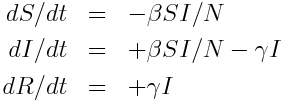
Where “S”, “I”, and “R” are the number of people in the population that are susceptible, infected and recovered.  The parameter “beta” is known as the transmission rate, and is the contact rate times the probability of transmission of infection on contact. Each susceptible person contacts beta people per day, a fraction I/N of which are infectious; thus beta*S*I/N is the flow out of the susceptible compartment, and into the infected compartment. The transmission rate is the average rate of contacts a susceptible person makes that are sufficient to transmit infection.  The last part of that sentence is important, because not all contacts a person makes with an infectious person are the type of contacts that will lead to infection; for instance, flu can be spread with casual contact, but a disease like AIDS requires quite intimate contact, thus b for AIDS is much smaller than that of flu.   The parameter “gamma” is known as the recovery rate, and gamma*I is the flow out of the infected compartment, and into the recovered compartment.  The average time a person spends in the infected class is 1/gamma days, and is usually estimated from observational studies of infected people.  For flu 1/gamma is around 3 days.

Notice that the model in the above equations does not include births or deaths, immigration or emigration. It also assumes that the transmission rate is constant, which is probably not a good assumption for diseases like influenza which have a much higher incidence in the winter than any other time of year.

Numerically solving the SIR model system of equations in R

Note that the system of ordinary differential equations above cannot be solved for S, I and R analytically.  Instead numerical methods must be used to numerically solve the model (such as Euler’s method, or Runge-Kutta).  In this module, I talk about both methods.

This is a nice website that discusses SIR modelling of influenza, and how to solve the system of equations using Euler’s method (also known as a time-difference method).  The R programming language has a nice package called deSolve that will solve systems of ODE’s using Runge-Kutta methods.  All you need to do is provide a function that calculates the derivatives. If you haven’t already previously installed deSolve into R on your computer, you can install it by typing

install.packages("deSolve")

in the R console (then pick a mirror site close to your location for the download).

An aside: deSolve is an example of a “Black Box”

Many applied mathematicians use the R deSolve library to numerically solve their models, or equivalent methods in Matlab (like ode45), or Mathematica, etc.  However, many never actually give a thought as to what is going on inside that code… they simply trust that it will spit out the correct answer.  In computing, any code that is simply viewed in terms of its inputs and outputs with no knowledge of its inner workings is termed a “black box.”

Black boxes, and the lack of understanding of their inner workings, can have many pitfalls.  In the case of numerically solving systems of ODE’s, if the ODE’s are stiff (for example, with parameters that might change dramatically in a short period of time), methods like deSolve will readily spit out an answer, but it should not be trusted.  The default time step used in the numerical integration is simply too coarse to adequately simulate the short term changes in the system.   And unless you were aware of the limitations of the methodology, you would never know that.

Unfortunately, there are many dazzlingly enticing software packages out there that do many fancy things, like parameter fitting, stochastic modelling, etc.  They can have wonderful sounding names that can lead to high expectations for their performance (like “self-adaptive genetic algorithms”, or “particle swarm optimisation”, as just a couple of examples).

Through long experience, I have a deep mistrust of black box code.  If I think a method might have some merit, I code up the algorithm myself, which also has the advantage that I gain a much deeper understanding of the methodology and its advantages and limitations.  Not infrequently, in doing this and after performing cross-checks on my code, comparison to the black box package shows that the black box code has bugs.

Now you know what deSolve does (and you can even code up versions of it yourself in R), and you are now aware of some of its limitations, so it is no longer a black box to you.  But hopefully this example will make you think a bit more deeply about any code you might just have otherwise used without a second thought as to how it goes about its inner calculations.

R code to model an influenza pandemic with an SIR model

Anyway, back to our ODE model example….

Let’s illustrate how to use R to model an influenza epidemic with an SIR model.  In the file sir_func.R I provide a function that calculates the time derivatives of S, I, and R using the equations above.  In the R script file sir.R I use that function when solving the model system of differential equations by using lsoda in the R deSolve package (note that sir.R also requires the R sfsmisc package, which you can install from the R console just like you installed deSolve, above).  Take some time to read through both files.  They are both heavily commented, so should be relatively self-explanatory.

Download sir_func.R and sir.R to your working directory in R.  Note to Windows users: ensure that Windows doesn’t sneakily append “.txt” to the end of the file, otherwise the instructions below will not work (ie; don’t save it as a text file in Windows, otherwise Windows adds a hidden “.txt” at the end of the file name). 

Also, for users of all operating systems, save the files with names exactly as I have them here.

To run the sir.R script, first change the working directory in R to the directory into which you’ve downloaded sir_func.R and sir.R by clicking on the

Misc->Change Working Directory

tab in the R toolbar, and selecting the directory you want in the drop down menu.  You can also set the working directory by typing into the R console*

setwd("<path name of your directory>")

Now type

source("sir.R")

and the following plot should appear**:

For this simulation I assumed a population size of 10 million, with one infected person introduced at time t=0.  I assume this is pandemic influenza with R0=1.5

Incidence is the number of new cases per unit time (usually by day, week or month), and is the data normally recorded during an epidemic (it is also the negative of the change in S during the time period). Prevalence is the fraction of the population infected at any point in time, and is the same as I. You see that prevalence reaches a maximum, then declines. The SIR epidemic eventually begins to wane because more and more of the population recovers and becomes immune.  From simple calculus, we know that dI/dt=0 when prevalence is at a maximum (or at a minimum), and if you examine the equations above, you see this will occur when S/N=gamma/beta.  It turns out that beta/gamma is the reproduction number (for more information on that, see the Mathematical Epidemiology book I refered to above), so the epidemic will peak when s=1/R0.

I denote on the plot the point where S=1/R0=2/3.  You can see that this is indeed the point where the prevalence peaks.  You can also see the initial exponential rise region in the bottom plot.

The sir.R script also outputs the fraction of susceptibles left in the population at the end of the epidemic, s_∞, as determined by the numerical model simulation.  This quantity can be determined via mathematical analysis of the model and the numerical solution to

-log(s_∞) = R0*(1-s_∞)

(assuming the initial population is entirely susceptible).  The code near the bottom of sir.R shows how to determine the numerical solution to that equation.

*If you have problems setting the working directory in the Windows operating system, the problem could be in how directory paths are written in R: make sure you use forward slashes in the directory path name, instead of the backward slash you are used to using in Windows.  So, an example of using setwd in R running in Windows is setwd(“C:/Users/mydirectory/”)

**If you have problems running the scripts, ensure that your working directory in R is the same as the directory where the scripts reside.  If using Windows, double check to ensure that the files haven’t been saved as “text” files, to which Windows appends a hidden “.txt”.

Further things you can explore

You can edit the sir.R script to try different population sizes and values of R0 and gamma, and rerun it to get a feeling for how these parameters affect the shape of the epidemic curve and the final size of the epidemic.  Also try different initial values for the fractions of susceptibles and infectives in the population.

You can also examine the sir_with_vaccination.R script, which includes a vaccinated compartment in the model, and moves susceptibles to the vaccinated compartment with rate rho during a specific time period: beginning with time_vaccination_begins, and ending with time_vaccination_ends.  The script models a hypothetical influenza epidemic, and examines two different vaccination strategies (rho=0.005 and rho=0.010 fraction vaccinated/day), and produces the plot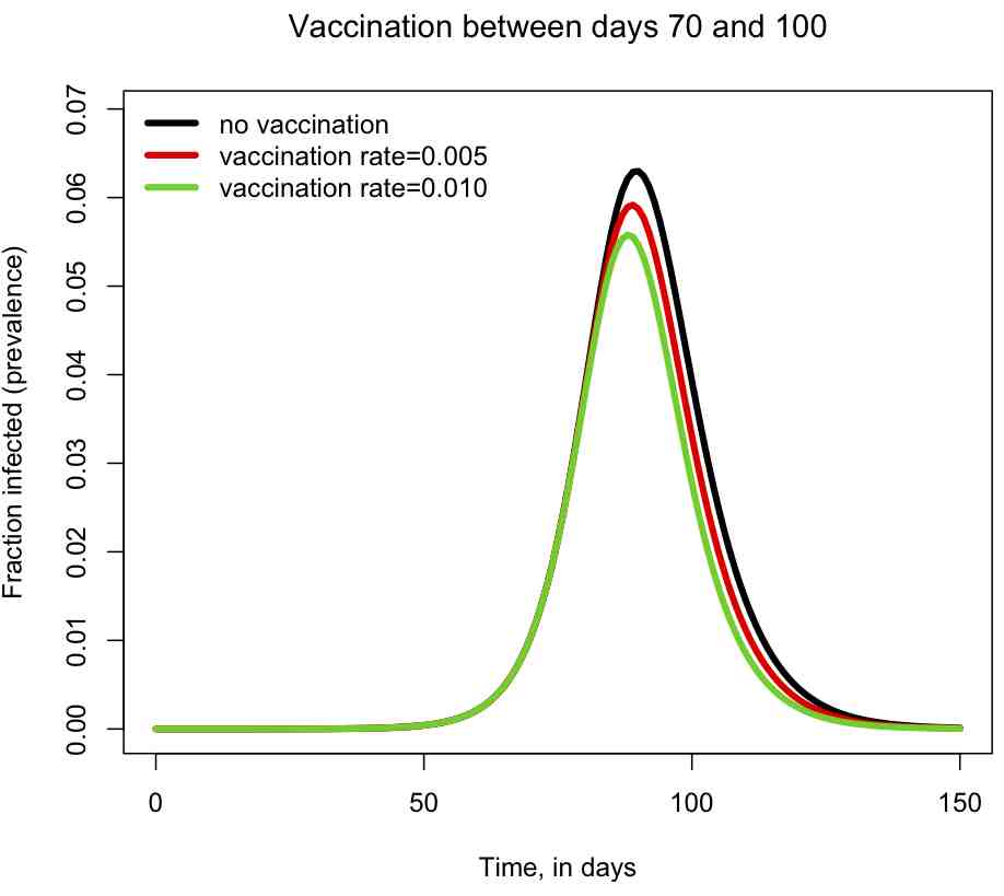

The script also prints out the fraction of the population that has been infected by the end of the epidemic.  You can try changing the vaccination period and the vaccination rates, and see how it affects the size of the epidemic, and the shape of the epidemic curve.

Summary

SIR models are remarkably effective at describing the spread of infectious disease in a population despite the many over-simplifications inherent in the model. For example, the model assumes homogenous mixing, but in reality a good fraction of the people we contact each day are always the same (ie; family members, class mates, co-workers, etc).  There are many different bells and whistles that can be added on to a simple SIR model to make it better describe the underlying dynamics of disease spread.  In future posts I will be talking about some of these, such as adding population age structure, adding time dependent transmission rates, etc.