[In this module, students will learn how to calculate the time step needed when applying numerical solution methods, such as the Runge-Kutta or Euler’s method, to solve systems of ODE’s associated with compartmental models.  This is not only useful knowledge for obtaining deterministic solutions, but also for stochastic modelling methods like Markov Chain Monte Carlo (MCMC), Stochastic Differential Equations (SDE’s), and Agent Based Models (ABM’s)].

It’s easy!

For any compartmental model, to get the average time needed to obtain an average change of a total of one individual in the model compartments, simply sum up the flows out of each compartment at that point in time, and then take the inverse (note that births are included in this calculation as a flow “out” of a compartment, even though they are really flowing in). 
For instance, here is the compartmental diagram and the equations for the SIR model:

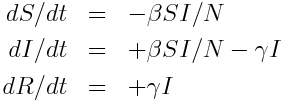
The flow out of the S compartment at time t is beta*S*I/N.  The flow out of the I compartment is gamma*I.  There is no flow out of the R compartment.  Thus our estimate of the time step needed to achieve an average change of one individual in the model compartments is

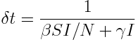   Eqn 1

Why does this work?  Notice that the units of delta_t are time per individual.  The units of beta*S*I/N and gamma*I are individuals per unit time.  The total number of individuals per unit time expected to change compartments is thus beta*S*I/N+gamma*I.  Taking the inverse of that yields the change in time per one individual.

Notice that as the number in the model compartments changes, so too does the number expected to leave the compartments per unit time, and thus so too does delta_t.  If the number leaving the compartments is large (for instance, near the peak of the epidemic in a SIR simulation) delta_t will be small.  When using numerical methods like Runge-Kutta or Euler’s method to solve systems of ODE’s either deterministically or stochastically, you should dynamically calculate the time step to achieve good accuracy in the numerical solution. If your model has vital dynamics in it (births and deaths), the number of births and deaths per unit time needs to be added to the denominator of delta_t. 

The R script seir_with_dynamic_time_step.R solves an SEIR model with vital dynamics using the 4th order Runge Kutta methods in the R deSolve library, and also using Euler’s method with a dynamically calculated time step.  It begins with a population of 1000 and simulates an influenza like illness spreading in the population.  It assumes that individuals leave the population after an average of 30 days; this could mean that the average lifespan of the individuals is 30 days, or it could mean that individuals just leave that particular population. For instance, with 1/mu~30 days this kind of model might be used to simulate the spread of influenza in a population like a county jail where people don’t (usually) die, but do have relatively short stays. 

Running the script produces the following plot overlaying the results from the two methods (try changing the population size to see how the results change):

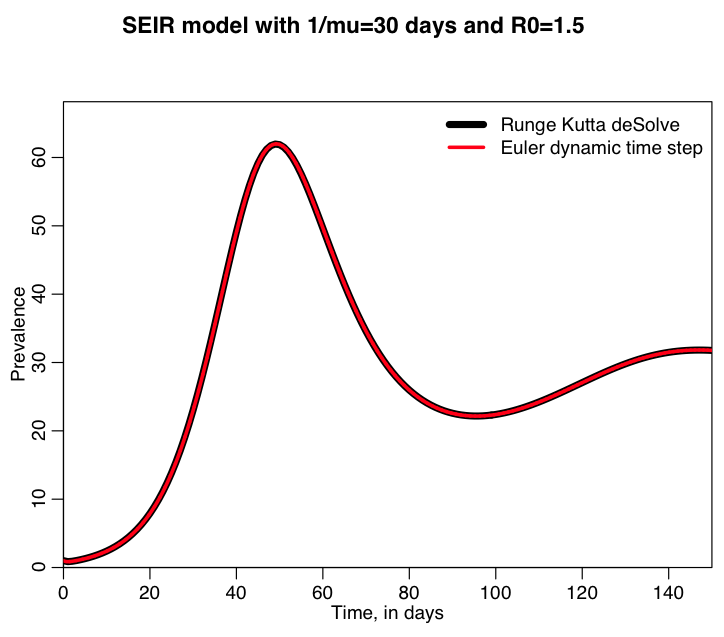
Try extending the simulation for a longer time period.  What do you notice, and what does this potentially imply for something like influenza in a jail population? How about if you change 1/mu from something short (like 30 days), to something longer (like years)?

Some finer points

When using a dynamic time step in your numerical simulations, you need to be aware that finding the average time step for, on average, one individual to change compartments may not be quite small enough to ensure accurate results. If you use too large a time step, the errors are cumulative, and your calculated model will diverge further and further from the true solution as you go forward in the simulation.

The problem is that the expected time for that to occur is exponentially distributed, with average delta_t.  The exponential distribution has very long tails, thus the median of the distribution is lower than the mean; thus 50% of the time, the time needed for an average of one individual to change compartments is actually less than what you calculated for delta_t (like, for instance for the SIR model in Eqn 1 above).  It is pretty straightforward to show with integration that for the exponential distribution with mean delta_t, a fraction p of the integrated distribution lies between 0 and log(1/(1-p))*delta_t.  Thus the median lies at log(2)*delta_t, and the 10th percentile lies at log(10/9)*delta_t. I err on the safe side, and use a small-ish percentile of the exponential distribution in my calculation of delta_t.  Like, for instance, the 10th or 25th percentile.  Especially when using Euler’s method, because it is inherently less accurate than the 4th order Runge Kutta method, and you need a small time step to achieve better accuracy.