
In this module, students will become familiar with Poisson regression for count data. We focus on the R glm() method for linear regression, and then describe the R optim() method that can be used for non-linear models.
The Poisson probability distribution is appropriate for modelling the stochasticity in count data. For example, like the number of people per household, or the number of crimes per day, or the number of Ebola cases observed in West Africa per month, etc etc etc.
There are other probability distributions that can be used to model the stochasticity in count data, like the Negative Binomial distribution, but the Poisson probability distribution is the simplest of the discrete probability distributions. The Poisson probability mass function for observing k counts when lambda are expected is:
The lambda is our “model expectation”, and it might be just a constant, or a function of some explanatory variables.
For example, perhaps we are examining how the number of crimes per day, k, might linearly depend on the daily average temperature, x. In this case, our model equation for lambda might be
![]()
where beta_0 and beta_1 are parameters of the model. But note that temperature can be negative, which might lead to negative values of the model expectation… clearly for count data this makes no sense!
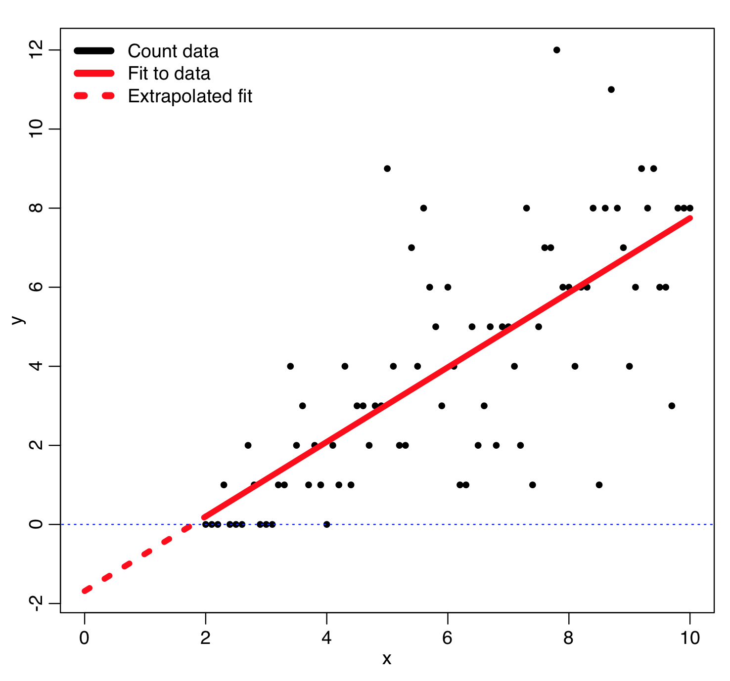
An example of how using least squares linear regression can go horribly wrong with count data for this reason is given by the following code, which reads in some count data, y, vs an explanatory variable, x, from the file example_of_how_least_squares_fits_to_count_data_can_go_wrong.csv
adat=read.table("example_of_how_least_squares_fits_to_count_data_can_go_wrong.csv",header=T,sep=",",as.is=T)
b = lm(y~x,data=adat)
mydat = data.frame(x=seq(0,2,0.1))
mydat$ypred = predict(b,mydat)
require("sfsmisc")
mult.fig(1)
xmin = min(c(adat$x,mydat$x))
xmax = max(c(adat$x,mydat$x))
ymin = min(c(adat$y,mydat$ypred))
ymax = max(c(adat$y,mydat$ypred))
plot(adat$x,adat$y,xlim=c(xmin,xmax),ylim=c(ymin,ymax),xlab="x",ylab="y")
lines(x,b$fit,col=2,lwd=5)
lines(mydat$x,mydat$ypred,col=2,lwd=5,lty=3)
lines(c(-1e6,1e6),c(0,0),lty=3,col=4)
legend("topleft",legend=c("Count data","Fit to data","Extrapolated fit"),col=c(1,2,2),lty=c(1,1,3),lwd=6,bty="n")
This produces the following plot… you can see that the extrapolated least squares fit predicts negative counts, which is impossible!
Solution…
With Poisson regression, we thus almost always use what is known as a “log-link” where we assume that the logarithm of lambda depends on the explanatory variables… this always ensures that lambda itself is greater than zero no matter what beta_0, beta_1 or x are:
![]()
Now, we might not know what beta_0 and beta_1 are, but if we have a bunch of observations of crimes over a series of N days, k_i (with i=1,…,N), and we also have for the same days, the average daily temperature, x_i, we can fit for beta_0 and beta_1 to determine which values best describe the observed relationship between the x_i and y_i. Our model for the expected number of crimes on the i^th day is thus
![]()
Using our collected data, we’d like to somehow estimate the “best-fit” values of beta_0 and beta_1 to the data. If the number of crimes per day is low, we can’t use least squares linear regression to do this because that method assumes that the data are Normally distributed, and it is only for large values of lambda that the Poisson distribution approaches the Normal.
We thus need a “goodness of fit” statistic that is appropriate to Poisson distributed data….
Poisson likelihood
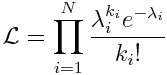
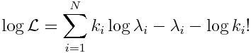
The likelihood (probability) of observing our data, k_i, given our model predictions for each data point, lambda_i, is the product of the probabilities of observing each data point separately:
 Eqn 1
Eqn 1
Our “best fit” values of lambda_i for this model are the ones that will maximize this probability. The least squares goodness-of-fit statistic is one that is usually quite easy for students to visualize. Likelihood fit statistics, however, are often more difficult to conceptualize because there isn’t a nice visual diagram that can explain it (like the arrows showing the distance between points and a model prediction, like we showed for least squares regression, for example).
However, for non-Normally distributed data, if you know what probability distribution underlies the data, you can write the likelihood distribution for observing a set of data by taking the product of the individual probabilities obtained from the probability distribution, just like we did above. The “best-fit” model maximizes that probability.
Fitting for the model parameters with Poisson likelihood
Note that probabilities that are multiplied in Eqn 1 are always between 0 and 1, and thus for a sample size of N points, Eqn 1 involves multiplying N values between 0 and 1 together. This can easily lead to underflow errors in our computation, which is a real problem for us when we try to apply this in practice. The solution to this is to take the logarithm of both sides of Eqn 1. Before we do that, here is a bit of a refresher on logarithms:
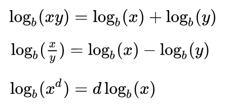
That is to say, the log of a product is the sum of the logs of the terms in the product. The log of x to some power is the same as that power times the logarithm of x. In this case, we will be taking the “natural log” (which is log_e, log to the base e) of both sides of Eqn 1. The natural log of e is log(e) = 1. Taking the natural logarithm of both sides of Eqn 1 thus yields:
 Eqn 2
Eqn 2
Poisson regression has been around for a long time, but least squares regression methods have been around longer. Finding the best-fit in least squares regression involves finding the parameters that minimize the least squares statistic. But finding the best-fit in Poisson regression involves finding the parameters in lambda_i that maximize Eqn 2. The interior gut workings of an optimization method in any statistical software package always minimize goodness of fit statistics, mostly because of the least squares legacy.
Because of this, we take the negative of both sides of Eqn 2, and we say that the best-fit parameters in Poisson regression minimize the negative log likelihood:
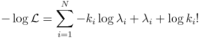
For the special case of our linear model for log(lambda_i) that we are considering, we get:
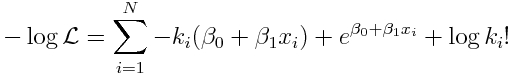 Eqn 3
Eqn 3
Given some data k_i and x_i, the “best-fit” values of beta_0 and beta_1 minimize that expression. We could, in practice, guess a whole bunch of different values for beta_0 and beta_1, and plug them into Eqn 3, and narrow it down to which pair of values appear to give the smallest negative log likelihood. However, principles of calculus can be used to find the best fit values of beta_0 and beta_1 that minimize the expression in Eqn 3. These methods are used in the inner workings of the R least squares linear regression lm() function, which is used when the response variable is Normally distributed. When working with a linear regression model with Poisson distributed count data, the R generalized linear model method, glm(), can be used to perform the fit using the family=”poisson” option. Just like with the R least squares method, invisible to you the inner workings of the glm() methods use calculus principles to find the best-fit model parameters that minimize the Poisson negative log likelihood. If the response data (our k_i) are in a vector y, and our explanatory variable, x_i, is in a vector x, and we are fitting a linear Poisson model, the function call looks like this:
myfit = glm(y~x,family="poisson")
Note that even though a log-link hasn’t been specified for the linear model, that is in fact what the glm() model with family=poisson by default assumes.
Example
Let’s try fitting some simulated data with the glm() method with family=”poisson”. The following code randomly generates some Poisson distributed data, with a linear model with a log-link:
########################################################################
# randomly generate some Poisson distributed data according to a linear model
########################################################################
set.seed(484272)
x = seq(0,100,0.1)
intercept_true = 1.5
slope_true = 0.05
log_lambda = intercept_true+slope_true*x
pred = exp(log_lambda)
y = rpois(length(x),pred)
########################################################################
# put the data in a data frame
########################################################################
mydat=data.frame(x=x,y=y)
Now let’s fit a linear model to these simulated data, under the assumption that the stochasticity is Poisson distributed. Note that the plotting area is divided up with the mult.fig() method in the R sfsmisc library. You need to have this library installed in R to run that line of code. If you don’t have it installed, first type install.packages(“sfsmisc”) and pick a download site relatively close to your location.
########################################################################
# Do the model fit using glm. Note that glm() with family="poisson"
# inherently assumes a log-link to the data
########################################################################
myfit_glm = glm(y~x,family=poisson,data=mydat)
print(summary(myfit_glm))
########################################################################
# Now plot the data with the fitted values overlaid. Note that
# even though the glm() method with family=poisson assumes a
# log-link, what it spits out in the fitted.values attribute
# is exponenent of that log-link
########################################################################
require("sfsmisc")
mult.fig(4,main="Poisson simulated data, generated with the model log(y)=a+b*x")
plot(x,y,xlab="x",ylab="y",cex=2,col="darkorchid4",main="y versus x")
lines(x,myfit_glm$fitted.values,col=3,lwd=5)
legend("topleft",legend=c("Simulated data","Best-fit Poisson linear model from R glm(y~x)"),col=c("darkorchid4",3),lwd=5,bty="n",cex=0.6)
plot(x,log(y),xlab="x",ylab="log(y)",cex=2,col="darkorchid4",main="log(y) versus x")
lines(x,log(myfit_glm$fitted.values),col=3,lwd=5)
The code produces the following output: 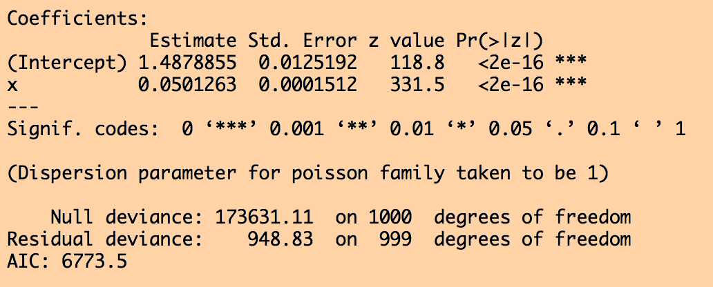
And the following plot: 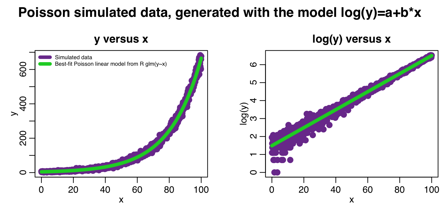
Are the fitted linear values statistically consistent with the true values we used to simulate the data? Do a z-test to check.
If I was presenting these results in a paper, I would say something along the lines of, “y is found to be significantly associated with x (Poisson linear regression coefficient 0.0501, with 95% CI [0.0507,0.0513] , p<0.001).”
Interpretation of the output
With a log-link linear model, log(y)=a+b*x, thus y=exp(a)*exp(b*x). You may wish to interpret the model results in terms of how a change in x from x=x_0 to x=2*x_0 changes y
We can see from the model that if x=x_0, y=exp(a)*exp(b*x_0), and if we double x, then x’=2*x_0 then y’=exp(a)*exp(2*b*x_0). Thus the relative change in y when we double x is y’/y=exp(b*x_0).
If b*x_0 is very small, then the first order Taylor expansion for y’/y~1+b*x_0. In fact, some readers may have been taught to use this expression for interpreting log-link Poisson regression results for the relative change in y. It needs to be stressed, however, that this interpretation only works if the coefficient b is small!
It is not just the R glm method with family=”poisson” that assumes a log-link for Poisson regression!
I’ve put this simulated data into a file simulated_poisson_log_linear_data.csv. If you have used other statistics software packages, like SAS, stata, SPSS, minitab, etc, try reading this data into that package and doing a Poisson linear regression fit. Compare the output of that software package to that you got in R. The coefficients and uncertainties should be the same. And what you should note in doing this exercise is that even though those other software packages may not specifically specify that the Poisson linear regression uses a log-link, they do.
The presentation in this module is not R specific: all Poisson linear regression uses a log-link by default.
Another example, with more than one explanatory variable
Let’s look at some real data…
The file chicago_crime_summary.csv contains the daily number of crimes in Chicago, sorted by FBI Uniform Crime Reporting code, between 2001 to 2013. FBI UCR code 4 is aggravated assaults (column x4 in the file). The file chicago_weather_summary.csv contains daily average weather variables for Chicago, including temperature, humidity, air pressure, cloud cover, and precipitation. The R script AML_course_libs.R contains some helper functions, including convert_month_day_year_to_date_information(month,day,year) that converts month, day, and year to a date expressed in fractions of years.
The following R code reads in these data sets, and meshes the temperature data into the crime data set. A few days are missing temperature data, so we remove those days from the data set. If you do not have the chron library already installed in R, first install it using install.packages(“chron”), and pick a download site close to your location.
require("chron")
cdat = read.table("chicago_crime_summary.csv",header=T,as.is=T,sep=",")
wdat = read.table("chicago_weather_summary.csv",header=T,as.is=T,sep=",")
cdat$jul = julian(cdat$month,cdat$day,cdat$year)
cdat$temperature = wdat$temperature[match(cdat$jul,wdat$jul)]
cdat$weekday = day.of.week(cdat$month,cdat$day,cdat$year)
cdat = subset(cdat,!is.na(cdat$temperature))
source("AML_course_libs.R")
a = convert_month_day_year_to_date_information(cdat$month,cdat$day,cdat$year)
cdat$date = a$date
To regress the daily number of assaults (the column x4 in the data frame) on temperature, we use the R glm() method with family=poisson:
myfit = glm(cdat$x4~cdat$temperature,family=poisson)
require("sfsmisc")
mult.fig(4,main="Daily assaults in Chicago, 2001 to 2013")
plot(myfit$fit,cdat$x4,xlab="Best-fit model prediction",ylab="Observed data")
lines(c(0,1e6),c(0,1e6),col=3,lty=3,lwd=3)
legend("topleft",legend=c("Hypothetical 'perfect' fit"),col=c(3),lwd=3,bty="n",cex=0.7)
plot(cdat$date,cdat$x4,xlab="Date",ylab="Daily \043 of assaults")
lines(cdat$date,myfit$fitted.values,col=2,lwd=3)
legend("topright",legend=c("Data","Best-fit model"),col=c(1,2),lwd=3,bty="n",cex=0.7)
This produces the following plot: 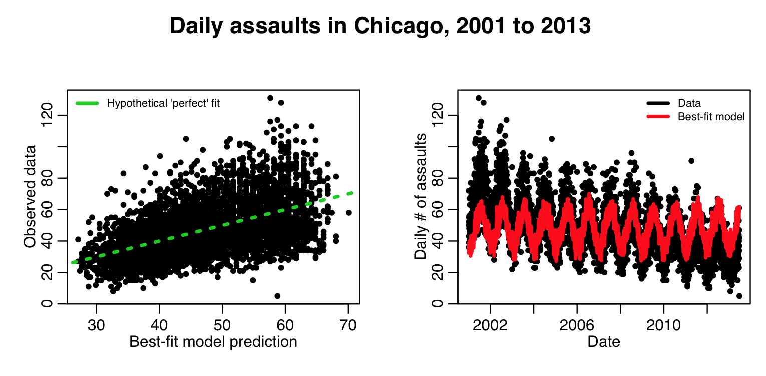
The fit clearly needs linear trend in time in order to fit the data better. The following code adds that:
myfit = glm(cdat$x4~cdat$temperature+cdat$date,family=poisson)
mult.fig(4,main="Daily assaults in Chicago, 2001 to 2013")
plot(myfit$fit,cdat$x4,xlab="Best-fit model prediction",ylab="Observed data")
lines(c(0,1e6),c(0,1e6),col=3,lty=3,lwd=3)
legend("topleft",legend=c("Hypothetical 'perfect' fit"),col=c(3),lwd=3,bty="n",cex=0.7)
plot(cdat$date,cdat$x4,xlab="Date",ylab="Daily \043 of assaults")
lines(cdat$date,myfit$fitted.values,col=2,lwd=3)
legend("topright",legend=c("Data","Best-fit model"),col=c(1,2),lwd=3,bty="n",cex=0.7)
This produces the following plot: 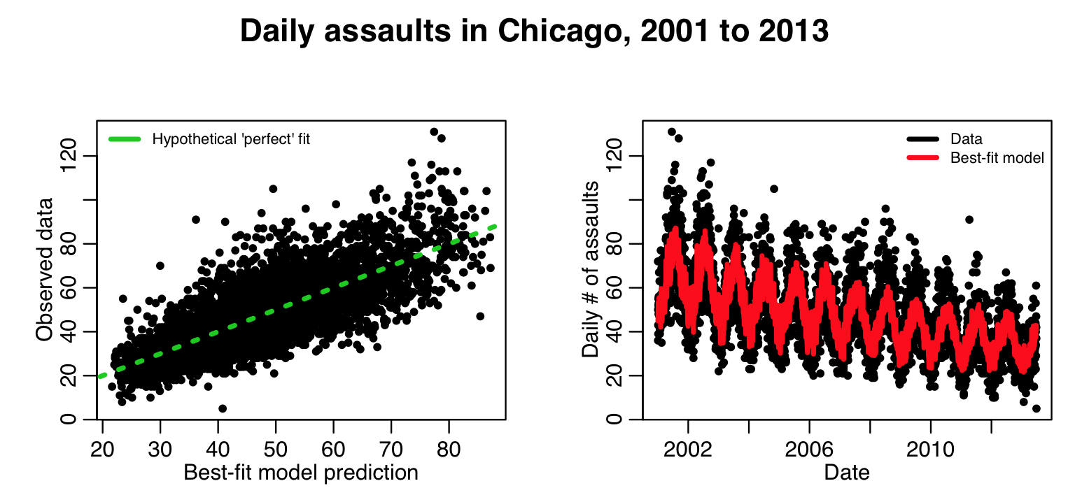
This looks to be a better fit.
But is the stochasticity in the data really consistent with being Poisson distributed? Just like the QQ plot we made with the Least Squares regression fits to test whether or not the data were truly Normally distributed about the model hypotheses, we can make a similar set of plots, but for the Poisson distribution. The AML_course_libs.R script contains a function
overlay_expected_distribution_from_poisson_glm_fit = function(count_data,glm_model_object)
that takes as its arguments the vector of count data, and the best-fit linear model from the glm() method.
In the first part of this function, for each data point it determines the shape of the probability mass function given the model prediction for that point… it then adds these mass functions up for all the data points. When we histogram the data, we can overlay this “Poisson model expectation” curve.
The second part of the script creates a QQ plot of the quantiles of the ranked data, vs the quantiles of a simulated data set, simulated assuming the best-fit model with Poisson stochasticity. If the data truly are Poisson distributed about the model, we would expect this plot to be linear. The following code implements this function with our data and our model to produce the plot:
overlay_expected_distribution_from_poisson_glm_fit(cdat$x4,myfit)
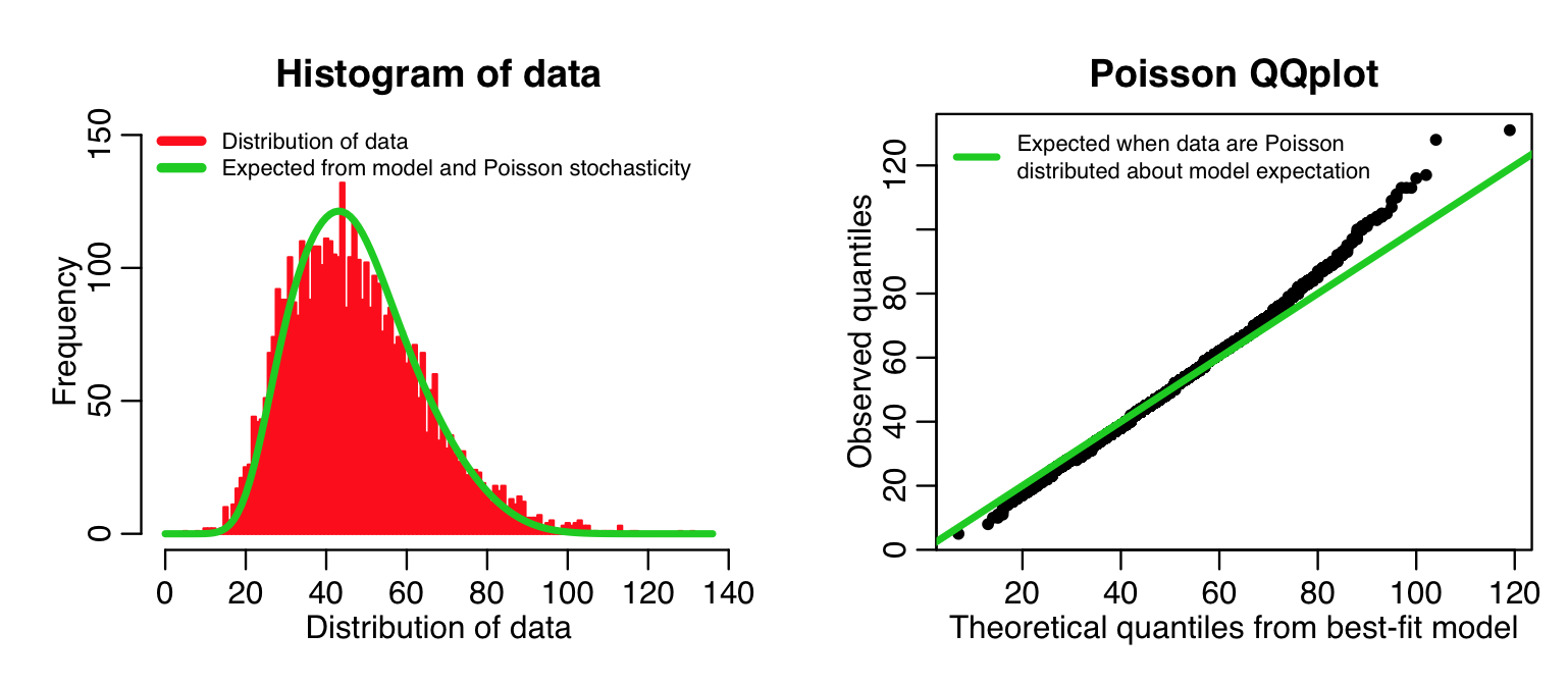
Even though our model with temperature plus linear trend in time is a better fit to the data than the model with just temperature, you can see that the above plots show that the data aren’t quite Poisson distributed about the model predictions. In fact, the QQ plot diagnostics indicate that the distribution appears to have some evidence of fat tails. This could point to potential confounding variables we haven’t yet taken into account (like, perhaps we might consider adding weekdays or holidays as factor levels in the fit). However, the data don’t appear to be grossly over-dispersed compared to the stochasticity expected from Poisson distributed data. Here is an example of including a factor in the explanatory variables (in this case weekday):
myfit = glm(cdat$x4~cdat$temperature+cdat$date+factor(cdat$weekday),family=poisson)
print(summary(myfit))
mult.fig(4,main="Daily assaults in Chicago, 2001 to 2013")
plot(myfit$fit,cdat$x4,xlab="Best-fit model prediction",ylab="Observed data")
lines(c(0,1e6),c(0,1e6),col=3,lty=3,lwd=3)
legend("topleft",legend=c("Hypothetical 'perfect' fit"),col=c(3),lwd=3,bty="n",cex=0.7)
plot(cdat$date,cdat$x4,xlab="Date",ylab="Daily \043 of assaults")
lines(cdat$date,myfit$fitted.values,col=2,lwd=3)
legend("topright",legend=c("Data","Best-fit model"),col=c(1,2),lwd=3,bty="n",cex=0.7)
overlay_expected_distribution_from_poisson_glm_fit(cdat$x4,myfit)
Model selection
Just like with least squares regression, it is important to select the most parsimonious model that gives the best description of the data. Every potential explanatory variable has stochasticity associated with it, and that extra stochasticity broadens the confidence interval on the fit parameters for all parameters.
If those variables actually don’t have any explanatory power, that added stochasticity can thus carry the risk of disguising significant relationships to truly explanatory variables.
As with least squares linear regression, we can use the Aikaike Information Criterion AIC statistic to compare how well models fit data, with a penalization term for the number of parameters, k:
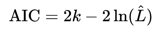
Note that the AIC includes the negative log likelihood… the smaller the negative log likelihood, the larger the likelihood. Thus, we want the most parsimonious model with the minimum value of the AIC.
The R stepAIC() function does model selection based on the AIC, dropping and adding terms in the candidate model one at a time, then calculating the AIC of the sub model.
After running the above code example, make sure the R MASS library is installed, and run the following code:
require("chron")
cdat = read.table("chicago_crime_summary.csv",header=T,as.is=T,sep=",")
wdat = read.table("chicago_weather_summary.csv",header=T,as.is=T,sep=",")
cdat$jul = julian(cdat$month,cdat$day,cdat$year)
source("AML_course_libs.R")
a = convert_month_day_year_to_date_information(cdat$month,cdat$day,cdat$year)
cdat$date = a$date
cdat$temperature = wdat$temperature[match(cdat$jul,wdat$jul)]
cdat$humidity = wdat$humidity[match(cdat$jul,wdat$jul)]
cdat$pressure = wdat$pressure[match(cdat$jul,wdat$jul)]
cdat$weekday = day.of.week(cdat$month,cdat$day,cdat$year)
cdat = subset(cdat,!is.na(cdat$temperature+cdat$humidity))
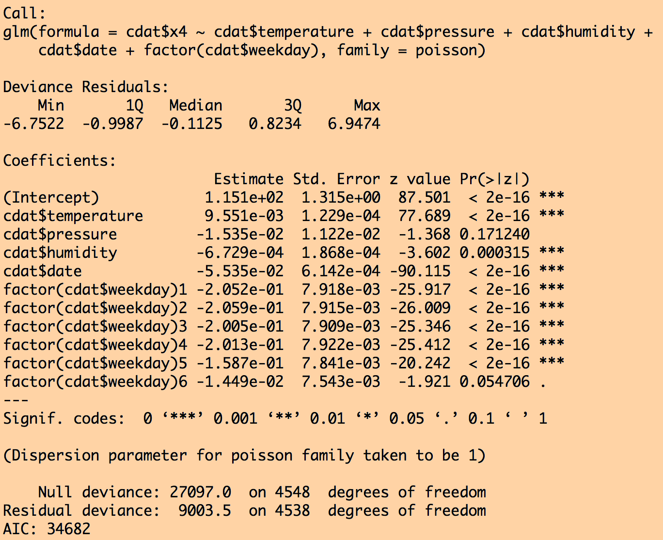
myfit = glm(cdat$x4~cdat$temperature+cdat$pressure+cdat$humidity+cdat$date+factor(cdat$weekday),family=poisson)
print(summary(myfit))
require("MASS")
d = stepAIC(myfit)
print(summary(myfit))
print(summary(d))
This produces the output:
and for the sub model fit selected by stepAIC():
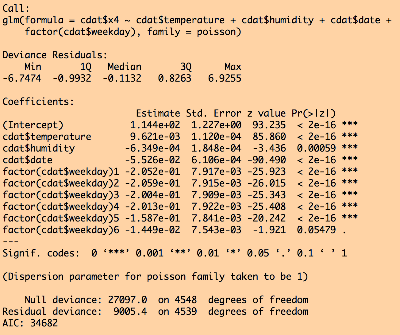
Notice that air pressure was dropped from the fit by stepAIC because that submodel had a lower AIC. Also notice that the standard error went down on all the other parameter estimates once air pressure was dropped.
Some cane waving…
 When I was a lass, working on my degree in experimental particle physics, we had to do model fitting very frequently. However, while we had a fortran (and later, a C++ package) that performed gradient descent optimization (or other optimization methods) of some function that you fed it, we didn’t have convenient pre-packaged methods like lm() or glm() where you could just fit a linear model with one tidy line of code. Instead, we had to write the code to actually program the likelihood ourselves.
 We also had to walk to school ten miles a day, barefoot, through waist deep snow, even in the summer, and it was uphill both ways.
Get off my lawn.
While it can be a pain to have to code up the actual likelihood expression, the advantage of that stone age methodology was that we had to think carefully about what kind of stochasticity underlay our data, and code up the appropriate likelihood function (or least squares expression, if the stochasticity was Normally distributed). Using canned methods in statistical software packages for doing fitting can unfortunately sometimes lead to decreased understanding of what’s really going on with the fit.
Believe it or not, particle physicists still do fitting the same way they always have, coding up the likelihood function themselves. And they probably always will. Because it is critically important when testing hypotheses that you not only have your model right (ie; accounting for all potential confounding variables, and ensuring that the functional expression of the model is appropriate), but that you also have the correct specification of the probability distribution describing stochasticity in the data. Otherwise your p-values testing your null hypothesis are garbage.
Getting up close and personal with Poisson regression in R
R has a method called optim() that finds the parameters that minimize the function you feed to it. Unlike the glm() method, which can only find the parameters of a linear model, the optim() method can find the parameters of any kind of model. For instructive purposes to show how optim() works, let’s code up the Poisson negative log likelihood using the optim() method, and use it to fit a linear model to some data, and compare what we get out of the glm() method with family=”poisson”. The two methods should yield the same results. Describing the optim() method also gives you a better idea of what R is doing inside the guts of the glm() method. The R script poisson_and_optim.R defines the following functions that define a linear model with a log-link, and also calculate the Poisson negative log likelihood, given some data vectors x and y contained in a data frame, mydata_frame.
########################################################################
########################################################################
# this is the function to calculate our linear model, assuming
# a log link
########################################################################
mymodel_log_prediction = function(mydata_frame,par){
 log_model_prediction = par[1] + par[2]*mydata_frame$x
 return(log_model_prediction)
}
########################################################################
########################################################################
# this is a function to compute the Poisson negative log likelihood
########################################################################
poisson_neglog_likelihood_statistic = function(mydata_frame,par){
 model_log_prediction = mymodel_log_prediction(mydata_frame,par)
 # lfactorial(y) is log(y!)
 neglog_likelihood = sum(-mydata_frame$y*model_log_prediction
 +exp(model_log_prediction)
 +lfactorial(mydata_frame$y))
 return(neglog_likelihood)
}
Now, we need some data to fit to. The R script also has code that simulates some data with Poisson distributed stochasticity according to a linear model with a log-link (same as the first example we showed above):
########################################################################
# randomly generate some Poisson distributed data according to a linear model
########################################################################
set.seed(484272)
x = seq(0,100,0.1)
intercept_true = 1.5
slope_true = 0.05
log_lambda = intercept_true+slope_true*x
pred = exp(log_lambda)
y = rpois(length(x),pred)
########################################################################
# put the data in a data frame
########################################################################
mydat=data.frame(x=x,y=y)
Now the script does the glm() fit, and the fit using the optim() method. The two methods return the results in an entirely different format, and it takes a bit more work to extract the parameter uncertainties using the optim() method:
########################################################################
# Do the model fit using glm. Note that glm() with family="poisson"
# inherently assumes a log-link to the data
########################################################################
myfit_glm = glm(y~x,family=poisson,data=mydat)
print(summary(myfit_glm))
coef = summary(myfit_glm)$coef[,1]
ecoef = summary(myfit_glm)$coef[,2]
cat("\n")
cat("Results of the glm fit:\n")
cat("Intercept fitted, uncertainty, and true:",round(coef[1],3),round(ecoef[2],5),intercept_true,"\n")
cat("Slope fitted, uncertainty, and true:",round(coef[2],3),round(ecoef[2],5),slope_true,"\n")
cat("Negative log likelihood:",-logLik(myfit_glm),"\n")
cat("\n")
########################################################################
# now do the R optim() fit
#
# The results of the fit are in much more of a primitive format
# than the results that can be extracted from an R glm() object
# For example, in order to get the parameter estimate uncertainties,
# we need to calculate the covariance matrix from the inverse of the fit
# Hessian matrix (the parameter uncertainties are the square root of the
# diagonal elements of this matrix)
# Also, if we want the best-fit estimate, we need to calculate it
# ourselves from our model function, given the best-fit parameters.
########################################################################
myfit_optim = optim(par=c(1,0),poisson_neglog_likelihood_statistic,mydata_frame=mydat,hessian=T)
log_optim_fit = mymodel_log_prediction(mydat,myfit_optim$par)
coef = myfit_optim$par
coefficient_covariance_matrix = solve(myfit_optim$hessian)
ecoef = sqrt(diag(coefficient_covariance_matrix))
cat("\n")
cat("Results of the optim fit:\n")
cat("Intercept fitted, uncertainty, and true:",round(coef[1],3),round(ecoef[1],5),intercept_true,"\n")
cat("Slope fitted, uncertainty, and true:",round(coef[2],3),round(ecoef[2],5),slope_true,"\n")
cat("Negative log likelihood:",myfit_optim$value,"\n")
cat("\n")
This produces the following output: 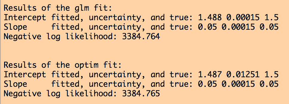
The following code overlays the fit results from both methods on the data:
########################################################################
# Now plot the data with the fitted values overlaid. Note that
# even though the glm() method with family=poisson assumes a
# log-link, what it spits out in the fitted.values attribute
# is exponenent of that log-link
########################################################################
require("sfsmisc")
mult.fig(4,main="Poisson simulated data, generated with the model log(y)=a+b*x")
plot(x,y,xlab="x",ylab="y",cex=2,col="darkorchid4",main="y versus x")
lines(x,myfit_glm$fitted.values,col=3,lwd=5)
lines(x,exp(log_optim_fit),col=2,lwd=1)
legend("topleft",legend=c("Simulated data","Best-fit Poisson linear model from R glm(y~x)","Best-fit Poisson linear model from R optim()"),col=c("darkorchid4",3,2),lwd=5,bty="n",cex=0.6)
plot(x,log(y),xlab="x",ylab="log(y)",cex=2,col="darkorchid4",main="log(y) versus x")
lines(x,log(myfit_glm$fitted.values),col=3,lwd=5)
lines(x,log_optim_fit,col=2,lwd=1)
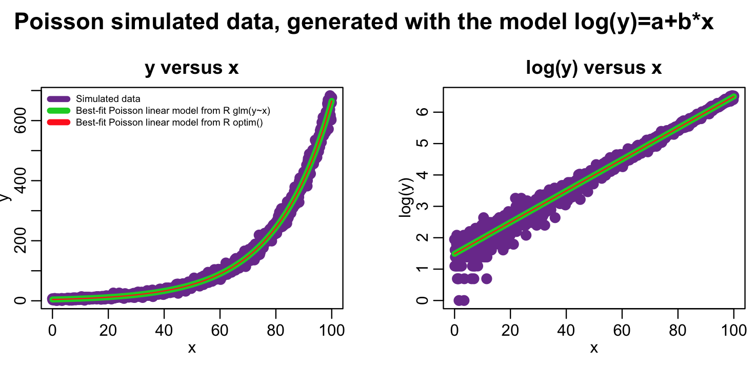
In this case we just did a simple linear model fit. However, with changes to the mymodel_log_prediction() method, optim() can fit arbitrarily complicated models, including non-linear models. Unlike optim(), the glm() method cannot fit non-linear models.