
In this module, students will become familiar with logistic (Binomial) regression for data that either consists of 1’s and 0’s (“yes” and “no”), or fractions that represent the number of successes out of n trials. We focus on the R glm() method for logistic linear regression.
The Binomial probability distribution is appropriate for modelling the stochasticity in data that either consists of 1’s and 0’s (where 1 represents as “success” and 0 represents a “failure”), or fractional data like the total number of “successes”, k, out of n trials.
Note that if our data set consists of n 1’s and 0’s, k of which are 1’s, we could alternatively express our 1’s and 0’s data as k successes out of n trials.
There are other probability distributions that can be used to model the stochasticity in fractional, like the Beta Binomial distribution, but the Binomial probability distribution is the simplest of the probability distributions for modelling the number of successes out of N trials. The Binomial probability mass function for observing k successes out of n trials when a fraction p is expected, is

The parameter p is our “model expectation”, can can be just a constant, or a function of some explanatory variables, and is the expected value of k/n.
Note that if our data are 1’s and 0’s, each point could be considered a “trial”, where k could be either 1 or 0 for each data point, and n would be 1 for each data point. This special case of the Binomial distribution is known as the Bernoulli distribution.
Our predicted probability of success, p, could, in theory at least, be a linear function of some explanatory variable, x:
![]()
However, this can present problems, because p must necessarily lie between 0 and 1 (because it is a fraction), but the explanatory variable might be negative, or even if it were positive, beta_0 and beta_1 might be such that the predicted value for p lies outside 0 and 1. This is a problem!
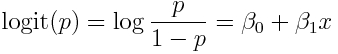
Partly for this reason, Binomial logistic regression generally assumes what is known as a “logit-link”. The logit of a fraction is log(p/(1-p)), also know as the log-odds, because p/(1-p) is the odds of success. It is this logit link that give “logistic regression” its name.
Note that because p lies between 0 and 1, p/(1-p) lies in the range of 0 to infinity. This means that the logit of p (the log of the odds) lies between -infinity to +infinity. With the logit-link, we regress the logit of p on the explanatory variables. For linear regression with one explanatory variable, this looks like:
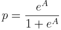
Because the logit lies in the range of -infinity to +infinity, now it doesn’t matter if the expression on the RHS of the equation is negative… the reverse transform will always give back a value of p between 0 and 1.
Nice!
By the way, if we call logit(p)=A, then the reverse transformation to calculate p is
Let’s assume that we have N data points of some observed data, k_i, successes, out of n_i trials, where i = 1,…N. This could be, for example, the daily n fraction of firearms the TSA detects that have a round chambered over a period of N days. k_i is the number each day found with a round chambered, and n_i is the total number found each day. The observed fraction might, at least hypothetically, linearly depend on time, x_i. In this case, our model looks like
![]()
In order to fit for beta_0 and beta_1 (or whatever the parameters of our model are), we need some “goodness of fit” statistic that we can optimize to estimate our best-fit values of our model with Binomially distributed data…
Binomial likelihood
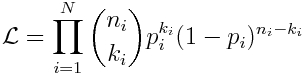
The likelihood of observing our N data points, k_i, out of n_i when p_i are expected for each point is the product of the individual Binomial probabilities:
 Eqn 1
Eqn 1
The “best-fit” parameters in the functional dependence of p_i on the explanatory variable, x_i (or variables… there doesn’t need to just be one), are the parameters that maximize this likelihood.
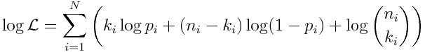
However, just like was pointed out in our discussion of Poisson regression methods for count data, in practice, underflow problems happen when you multiply a whole bunch of likelihoods (probabilities) together, each of which is between 0 and 1. To avoid this, what is normally done is take the logarithm of both sides of Eqn 1, and what is maximized is the logarithm of the likelihood, log(L):
The R glm() method with family=”binomial” option allows us to fit linear models to Binomial data, using a logit link, and the method finds the model parameters that maximize the above likelihood. If the success data is in a vector, k, and the number of trials data is in a vector, n, the function call looks like this:
myfit = glm(cbind(k,n-k)~x,family="binomial")
The glm() binomial method can also be used with data that are a bunch of 1’s and 0’s. For our little example here, the data might be at the individual firearm level, where ‘1’ indicates that the firearm has a round chambered, and ‘0’ indicates that it doesn’t. In this case, if the vector found_with_round_chambered contains these zeros and ones for all the firearms, and the vector day_gun_found contains the day each firearm was found (relative to some start day), we can fit to this data using the function call
myfit = glm(found_with_round_chambered~day_gun_found,family="binomial")
Note that in both cases, it is exactly the same data, just expressed a different way (you can always aggregate the 1’s and 0’s by day to get the total number of firearms found, and the number found with a round chambered each day, for example). This duality in how you can look at logistic regression is sometimes confusing to students who have been exposed to logistic regression methods either just using 0’s and 1’s, or just using fractional data.
Example
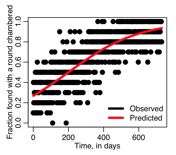
Let’s simulate some Binomial data, with trend in time. In the example described above, perhaps this might be firearms detected at TSA airport checkpoints, and determining whether they had a round chambered (“1”), or didn’t have a round chambered (“0”). In this simulated example, the logit of the fraction loaded, p, has the predicted trend
set.seed(541831)
vday = seq(0,2*365)
vlogit_of_p_predicted = -1+0.005*vday
vp_predicted = exp(vlogit_of_p_predicted)/(1+exp(vlogit_of_p_predicted))
At time vday=0, the predicted average fraction of firearms found with a round chambered is thus:
p=exp(-1)/(1+exp(-1)) = 0.269
At time vday=730, the predicted average fraction of firearms found with a round chambered is:
p=exp(-1+0.005*730)/(1+exp(-1+0.005*730)) = 0.934
Let’s simulate same data where we assume the TSA detects exactly 25 firearms per day. We’ll simulate the data at the firearm level, where we record the day each firearm was found, and if it had a round chambered:
num_guns_found_per_day = 10
wfound_with_round_chambered = numeric(0)
wday_gun_found = numeric(0)
for (i in 1:length(vday)){
  v = rbinom(num_guns_found_per_day,1,vp_predicted[i])
  wfound_with_round_chambered = c(wfound_with_round_chambered,v)
  wday_gun_found = c(wday_gun_found,rep(vday[i],num_guns_found_per_day))
}
Notice that the wfound_with_round_chambered vector contains 1’s and 0’s.
We can recast this data instead by aggregating the number found with and without a round chambered by day:
num_aggregated_ones_per_day = aggregate(wfound_with_round_chambered,by=list(wday_gun_found),FUN="sum")
 num_aggregated_zeros_per_day = aggregate(1-wfound_with_round_chambered,by=list(wday_gun_found),FUN="sum")
vday = num_aggregated_ones_per_day[[1]]
vnum_found_with_round_chambered = num_aggregated_ones_per_day[[2]]
vnum_found_without_round_chambered = num_aggregated_zeros_per_day[[2]]
vnum_found = vnum_found_with_round_chambered + vnum_found_without_round_chambered
Let’s plot the simulated data
vp_observed=vnum_found_with_round_chambered/vnum_found
plot(vday,vp_observed,cex=2,xlab="Time, in days",ylab="Fraction found with a round chambered")
lines(vday,vp_predicted,lwd=4,col=2)
legend("bottomright",legend=c("Observed","Predicted"),col=c(1,2),lwd=4,bty="n")
which produces the plot:
Now let’s do a linear logistic fit using the R glm() with family=”binomial” to the individual firearm data, and then to the data aggregated by day. When looking at aggregated data, we input the data to the fit as cbind(num_successes,num_failures). This can also be expressed as cbind(k,n-k), if k is num_successes, and n is the number of trials (n=num_successes+num_failures).
Note that the event and aggregated data are exactly the same data, so they should give exactly the same fit results!
fit_to_daily_data = glm(cbind(vnum_found_with_round_chambered,vnum_found_without_round_chambered)~vday,family="binomial")
fit_to_event_data = glm(wfound_with_round_chambered~wday_gun_found,family="binomial")
print(summary(fit_to_daily_data))
print(summary(fit_to_event_data))
This produces the output:


We can plot the fit results overlaid on the data. Note that even though glm() uses the logit link, it converts the fit prediction to a probability to save you the work of doing it.
plot(vday,vp_observed,cex=2,xlab="Time, in days",ylab="Fraction found with a round chambered")
lines(vday,vp_predicted,lwd=8,col=2)
lines(vday,fit_to_daily_data$fit,lwd=4,col=4,lty=3)
legend("bottomright",legend=c("Observed","True model","Fitted model"),col=c(1,2,4),lwd=4,bty="n")
Producing the plot:
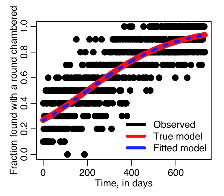
You can see that our fitted model is pretty close to the true model. This is because there are many data points (10 each day, for two years). If the data were much more sparse, we would expect to perhaps see a bit more deviation of the fitted model from the true, not because the true model is wrong (it is after all, the true model we used to simulate our data), but because with a sparse data set the fit gets more affected by stochastic variations in the data.
The script example_glm_binomial_fit.R does the above fit. You can try different values of number of guns found per day, and different model coefficients to see how it affects the simulated data and the fits.
Note that in this example we assumed a constant number of firearms found per day… we could have varied that, if we wanted, and it would not change the linear dependence of the logit of the probability of finding a firearm with a round chambered…. whether the number found per day is 1, or 100000 (or whatever), it doesn’t affect the probability of success.
Model selection
Just like least squares linear regression with the lm() method, or Poisson regression with the glm() method with family=”poisson”, you can use the R stepAIC() function to find the most parsimonious model that best fits the data.
A real life Binomial logistical analysis example
An inspection of the launch pad revealed large quantities of ice collecting due to unusually cold overnight Florida temperatures. NASA had no experience launching the shuttle in temperatures as cold as on the morning of Jan. 28, 1986. The temperatures of each of the 23 previous launches had been at least 20 degrees warmer.

At the launch site, the fuel segments were assembled vertically. Field joints containing rubber O-ring seals were installed between each fuel segment. There were three O-ring seals for each of the two fuel tanks.
The O-rings had never been tested in extreme cold. On the morning of the launch, the cold rubber became stiff, failing to fully seal the joint.
As the shuttle ascended, one of the seals on a booster rocket opened enough to allow a plume of exhaust to leak out. Hot gases bathed the hull of the cold external tank full of liquid oxygen and hydrogen until the tank ruptured.
At 73 seconds after liftoff, at an altitude of 9 miles (14.5 kilo- meters), the shuttle was torn apart by aerodynamic forces.
The two solid-rocket boosters continued flying until the NASA range safety officer destroyed them by remote control.
The crew compartment ascended to an altitude of 12.3 miles (19.8 km) before free-falling into the Atlantic Ocean, killing all aboard.
Decision to fly based on faulty analysis of data
This paper by Dalal, Fowlkes, and Hoadley (1989), described the O-ring failure data from the previous launches, and the reasoning behind the decision to launch on that cold day. The data from previous launches is shown in Table 1 of that paper, and I have put it in the file oring.csv
As it mentions in the Dalal et al paper, managers in charge of the launch decision felt that the launches with zero O-ring failures were non-informative of the risk of failure versus temperature, and thus excluded that data from their decision making process.
The following code reads in that data, and plots it against temperature:
o = read.table("oring.csv",sep=",",header=T,as.is=T)
o_without_zero = subset(o,num_failure>0)
require("sfsmisc")
mult.fig(1)
plot(o$temp,o$num_failure,cex=3,xlab="Temperature",ylab="\043 of O-ring failures",ylim=c(0,ymax),xlim=c(31,max(o$temp)),main="Space Shuttle O-Ring failure data for launches prior to Jan, 1986")
points(o_without_zero$temp,o_without_zero$num_failure,col="orange",cex=3)

The points in orange are the non-zero points that were used to make the decision to launch.
It is unclear what statistical acumen, if any, was used in the risk analysis that went into that decision, but it should be pointed out here that at least one person behind the scenes was very vocal about the mistake that was being made by ignoring the zero data prior to the launch.
Let’s assume, as an example, that the analysis methodology might have been at the Stats 101 level, and a least squares regression was attempted on the data (Note: why is this in fact a completely inappropriate method to use?)
b = lm(num_failure~temp,data=o_without_zero)
print(summary(b))
newdata = data.frame(temp=sort(c(o$temp,seq(30,70))))
ypred = predict(b,newdata,interval="predict")
cat("The expected number of O-ring failures at 31 degrees from the LS fit to num_failure>0:",ypred[newdata$temp==31,1],"\n")
ymax = 6
plot(o_without_zero$temp,o_without_zero$num_failure,cex=3,xlab="Temperature",ylab="\043 of O-ring failures",ylim=c(0,ymax),xlim=c(31,max(o$temp)),main="Least Squares Fit only to non-zero data")
lines(newdata$temp,ypred[,1],col=2,lwd=8)
lines(newdata$temp,ypred[,2],col=2,lwd=4,lty=3)
lines(newdata$temp,ypred[,3],col=2,lwd=4,lty=3)
legend("topright",legend=c("Least Squares fit","95% CI on fit prediction"),col=2,lty=c(1,3),lwd=4,bty="n")
(note that using interval=”predict” in the R predict() method will return not only the fit prediction, but also it’s 95% confidence interval that arises due to the uncertainty on the fit estimates)

From the fit summary, it is apparent that there is no significant slope wrt temperature (p=0.20). Thus, from a naive analysis like this, one might conclude that there is no significantly increased risk of O-ring failure at 31 degrees compared to 60 degrees.
How about if we redo the least squares regression, but this time including the zeros:
b = lm(num_failure~temp,data=o)
print(summary(b))
ypred = predict(b,newdata,interval="predict")
cat("The expected number of O-ring failures at 31 degrees from the LS fit to num_failure:",ypred[newdata$temp==31,1],"\n")
ymax = 6
plot(o$temp,o$num_failure,cex=3,xlab="Temperature",ylab="\043 of O-ring failures",ylim=c(0,ymax),xlim=c(31,max(o$temp)),main="Least Squares Fit")
lines(newdata$temp,ypred[,1],col=2,lwd=8)
lines(newdata$temp,ypred[,2],col=2,lwd=4,lty=3)
lines(newdata$temp,ypred[,3],col=2,lwd=4,lty=3)
legend("topright",legend=c("Least Squares fit","95% CI on fit prediction"),col=2,lty=c(1,3),lwd=4,bty="n")

The fit now shows a significantly negative slope (p<0.001), but the predicted number of O-ring failures at 31 degrees is less than three. Given that they already had at least one successful prior launch with two O-ring failures, this hardly looks like something to be necessarily worried about.
But wait… that fit predicts negative O-ring failures when the temperature is above around 75 degrees. That doesn’t make sense. And there are only 6 O-rings in total… if we were to extrapolate the fit to even lower temperatures, it’s clear that we would eventually predict more than 6 O-ring failures for very low temperatures.
Doing it right with Binomial logistic regression
The following code does the fit using Binomial logistic linear regression. You’ll need to download the file AML_course_libs.R to run this; it contains a method get_prediction_and_confidence_interval_from_binomial_fit that estimates the 95% interval on extrapolations of a Binomial regression fit.
source("AML_course_libs.R")
b = glm(cbind(num_failure,6-num_failure)~temp,family="binomial",data=o)
ypred = get_prediction_and_confidence_intervals_from_binomial_fit(b,newdata)
cat("The expected fraction of O-ring failures at 31 degrees from the logistic fit:",ypred[newdata$temp==31,1],"\n")
ymax = 1.0
plot(o$temp,o$frac,cex=3,xlab="Temperature",ylab="Fraction of O-rings that fail",ylim=c(0,ymax),xlim=c(31,max(o$temp)),main="Logistic regression")
lines(newdata$temp,ypred[,1],col=2,lwd=8)
lines(newdata$temp,ypred[,2],col=2,lwd=4,lty=3)
lines(newdata$temp,ypred[,3],col=2,lwd=4,lty=3)
legend("topright",legend=c("Logistic regression fit","95% CI on fit prediction"),col=2,lty=c(1,3),lwd=4,bty="n")
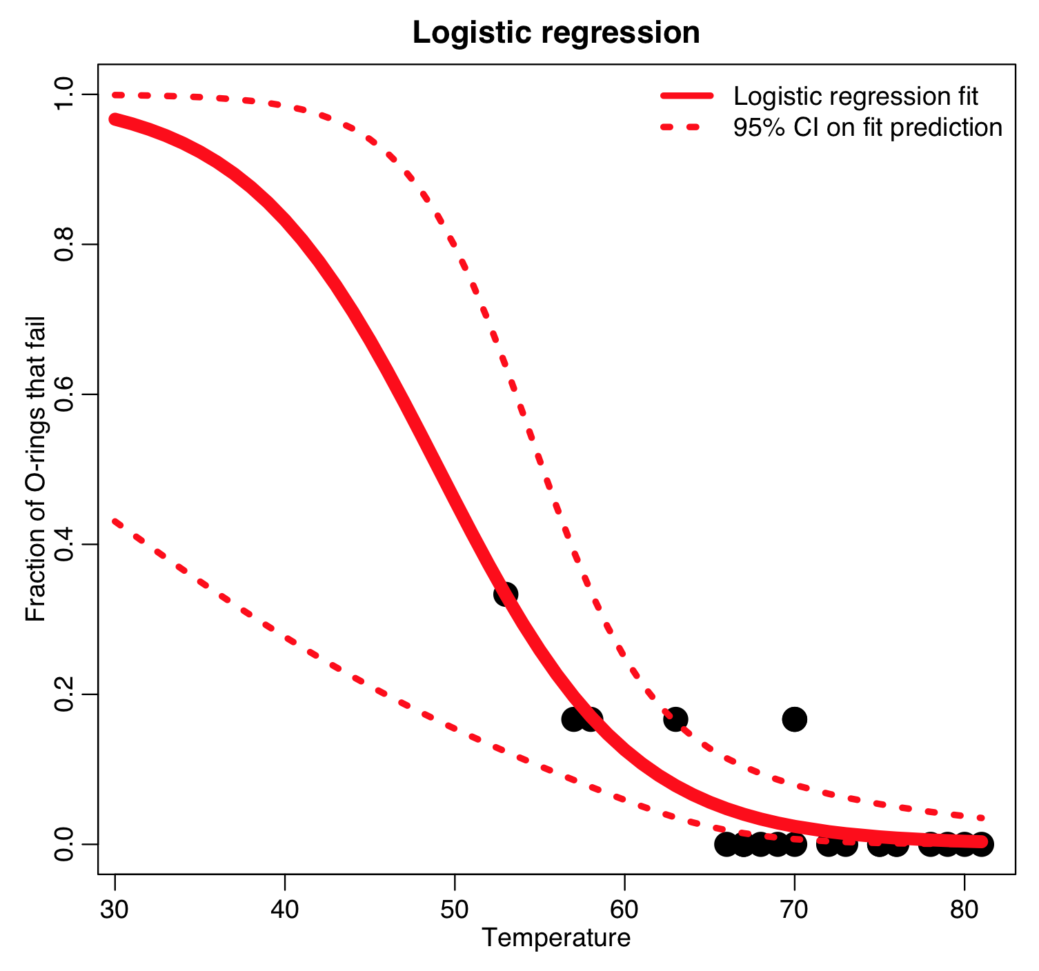
The y axis is the fraction of the O-rings that are expected to fail. The Binomial logistic regression predicts that 96% of the 6 rings will fail (ie; the likelihood is high that all 6 rings will fail). In fact, with 95% confidence, at least half of the rings will fail.
Beyond a statistical analysis of past launch data, however, apparently the O-rings had not been tested for flexibility at low temperatures. Richard Feynman, and Physics Nobel Prize laureate, was a member of the scientific commission that was appointed to look into the shuttle disaster. In a dramatic moment during the commission news conference, he demonstrated the inflexibility of O-rings at low temperature by pulling a deformed O-ring out of his glass of ice water.
Since the shuttle disaster, there have been other, more elaborate studies of the pre-launch O-ring data to attempt to assess the temperature dependent risk of failure…. for example, this analysis which examines the issue of model extrapolation given the large difference between the temperature of 31 degrees and all other temperatures in the past data, which were significantly warmer.
Moral of this story
Rare are statistical analyses we might attempt that might actually kill someone if we get it wrong. But this is an excellent case of how proper choice of analysis methods could have averted a disaster.