
In this module, students will become familiar with least squares linear regression methods. Note that before proceeding with any regression analysis, it is important to first perform initial data exploration, both with visualization analysis with histograms, boxplots, and scatter plots, and numerical summaries of the variables like the mean, standard deviations, maxima and minima, and correlations between variables. In this way, you can determine if there are any unexpected “quirks” or problems with the data (and, more often than not, there are).
Introduction
In this module we will be discussing fitting linear models to data, which is to say that we hypothesize that some relationship exists between our data, y, and some variable x that we think is likely linearly related (so our hypothesized model is y=a*x+b, and we wish to estimate the model parameters a and b).
One way we could do this is to try lots of different pairs of values of a and b, and choose the pair that appears to give us the “best fit” to the data. But in the field of statistical data analysis, assessing goodness of fit isn’t just done by looking at a plot of the data with the model overlaid and thinking “Yeah, that looks like the best fit so far…”. Instead, there are quantities (“figure or merit” statistics) that you can calculate that give an indication of how well the model fits the data. In this module, we will be discussing Least Square statistics for assessment of goodness of fit. The LS statistic is the sum of the squared distances between our data, y, and the model (in this case a*x+b).
Can you see that a well fitting model will be the one that minimizes the sum of these squared distances? Of the two models above, which looks like a better fit?
As an aside; looking at this data, do you think there is evidence of “significant” linear trend? Can you see that if there are fewer points that evidence of potential trend would be sketchier? Can you see if that the data have a lot of stochasticity (up and down variation from point to point) evidence of potential trend would also be sketchier? We will be discussing below the mathematical rigour of linear model fitting using least squares, and how to assess the significance of model parameters, testing the null hypothesis that they are consistent with zero.
Underlying assumptions of least squares regression
Before we move on to talk about the statistical details of linear models, an important aside that needs to be made is that Least Squares is just one goodness-of-fit statistic. Others exist (for instance weighted least squares, Pearson chi-square, or Poisson or Negative Binomial maximum likelihood). The different goodness-of-fit statistics assume different underlying things about the data. In the case of Least Squares, it assumes that all the data points have the same probability distribution underlying their stochasticity, and that probability distribution is Normal. This may or may not be a good assumption. The problem is that if this underlying assumption is violated, the Least Squares method will yield biased estimators for the model parameters, and also the p-values testing the null hypothesis that the parameters are consistent with zero will also be wrong.
Whatever fitting method we use, it is important to understand all of the underlying assumptions of the method, and ensure that the data actually are consistent with those underlying assumptions. Keep this in mind whenever you fit any kind of model to data, using any method.
Linear regression with Least Squares
Regression analyses are used to model the relationship between a variable Y (usually called the dependent variable, or response) and one or more explanatory (sometimes called independent) variables X1, X2, … Xp. When p>1 regression is also known as multivariate regression. When p=1 the regression is also known as simple regression.
In regression analyses, the dependent variable is continuous, but the explanatory variables can be continuous, discrete, or categorical (like Male/Female, for instance).
Regression analyses can be done for a variety of different reasons, for instance prediction of future observations, or assessment of the potential relationship between the dependent and independent variables.
Linear regression models assume a linear relationship between Y and one or more explanatory variables, and the parameters are obtained from the best fit to the data by optimizing some goodness of fit statistic like Least Squares. Thus the model for the linear dependence of the data y on one explanatory variable, x, would look like something like this for the i^th data point
![]()
where epsilon is a term that describes the left-over stochasticity in the data, after taking into account the linear regression line (epsilon is also known as the residual), and x_i are the data corresponding to the independent, explanatory variable, and the y_i are the data for the dependent variable. The alpha and the beta are the unknown parameters for which we will fit (and also epsilon, but we’ll get to that in a moment). Note that the equation is linear in those parameters, thus this is why it is known as linear regression.
The explanatory variables themselves can appear as non-linear functions, as long as unknown parameters don’t appear in the function. So, for a known frequency omega, and data points (t_i,y_i)
![]()
is also a linear model (and in fact, one that we will return to when we discuss harmonic linear regression later on in this AML 610 course to model periodic behaviour in the data). However, an example of a non-linear model when alpha and beta are unknown is:
![]()
In this course we will be focussing on linear regression rather than non-linear regression. However, not that sometimes with a bit of thought, you can transform a non-linear model into a linear model (for instance, if we knew alpha from prior information, in practice we could subtract it from Y and then take the log of both sides and use a linear model regression method to determine gamma and log(beta)).
Now, recall that if we are using Least Squares to determine our model parameters, the underlying assumption of that method is that the epsilon_i are all equal (a property known as homoscedasticity), with probability distribution Normal(mu=0,sigma=epsilon).
Now, note that if we have N data points, the y data can be more compactly expressed as a vector of length N. Similarly, the data for the independent variables can be expressed as a matrix. We can thus express the linear regression in matrix format as
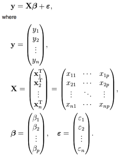
where p is the number of explanatory variables. X is often referred to as the “design matrix”.
Linear regression involves estimating values of beta that describe as much of the variation in the data as possible, by minimizing the sum of the squared residuals. The residuals are
![]()
where hat(y)_i is the predicted value of y_i from the linear regression model.
The left over variance is the sum of the squared residuals (RSS or SSE),
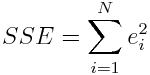
(note that N=n in the above equation). In the Least Squares method this is equal to
![]() Equation 2
Equation 2
To find the parameters that minimize the left-over variance involves simple calculus; we take the derivative of the LHS wrt the beta terms, then set it equal to zero. Plugging through the algebra yields that the values of beta that minimizes equation 2 is
![]()
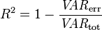
A measure of how much of the data variance is described by the model is known as R^2
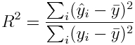
where bar(y) is the mean of the y vector (aside; note that the denominator in that expression is proportional to the variance of y). When R^2 is close to 1, then almost all the original variance in the data is described by the model (and the residual variance is very small).
Determination of the uncertainties on least squares linear regression parameter estimates
Because of the stochasticity in the data, there will be uncertainty in the estimates of beta. If there is a lot of stochasticity in the data and/or if there are just a few data points, the estimates of beta will have large uncertainties.
The covariance matrix for the parameters of a linear least squares model is
![]()
If V is this covariance matrix, the one standard deviation uncertainty on the first parameter is the square root of V[1,1]. The one standard deviation uncertainty on the second parameter (if there is more than one parameter being fit for) is the square root of V[2,2]. The correlation between those two estimated parameters is V[1,2]/sqrt(V[1,1]*V[2,2]).
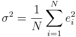
Where sigma^2 is the variance on the fit residuals, and is
The underlying probability distribution for a parameter estimate under the null hypothesis that it is equal to zero is Students-t with N-2 degrees of freedom. As N gets large, the Students-t distribution approaches the Normal distribution.
Questions: as N gets large (ie; lots of data), what happens to the uncertainties on the parameter estimates?
Linear regression in R with the lm() method
In practice, you will probably never have to do the above matrix arithmetic to calculate the parameter estimates of a linear model and their uncertainties; this is because software like R, Matlab, SAS, SPSS, Stata, etc all have linear regression methods that do it for you. In R, linear regression is done with the lm() method.
The lm() method outputs various fit diagnostics, including the parameter estimates, their uncertainties, and the p-value testing the null hypothesis that the parameter estimate is consistent with zero. It also outputs the R^2 of the model, and a statistic (called the F-statistic) that tests the null hypothesis that all model parameters except for the intercept are consistent with zero. These various diagnostics are accessed with the summary() function.
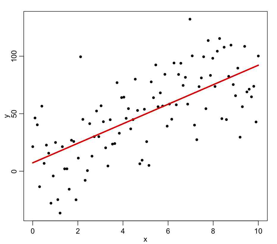
As an example, let’s generate some Monte Carlo simulated data with the underlying model y=10*x, and with underlying stochasticity epsilon~N(0,25). “Monte Carlo” means that random numbers are involved in the simulation.
Copy and paste the following into R:
require("sfsmisc")
set.seed(77134)
n = 100
x = seq(0,10,length=n)
intercept_true = 0
slope_true = 10
# Monte Carlo simulation of data y=a+c*x, with a=0 and c=10
y = intercept_true+slope_true*x+rnorm(n,0,25)
mydata = data.frame(x,y)

mult.fig(1)
plot(mydata,xlab="x",ylab="y")

myfit = lm(y~x,data=mydata)
lines(mydata$x,myfit$fitted.values,col=2,lwd=3)
The ~ in the above input to lm() means that whatever variable you put on the LHS is assumed to be described by the model on the RHS (which can involve one or more explanatory variables). When you run the above code, you will get the following plot:
Using summary(myfit) produces the following output:
summary(myfit)
Call:
lm(formula = y ~ x, data = mydata)

Residuals:
    Min      1Q  Median      3Q     Max
-55.718 -18.066   1.997  21.172  74.192

Coefficients:
            Estimate Std. Error t value Pr(>|t|)
(Intercept)   7.2908     5.3357   1.366    0.175
x             8.4868     0.9218   9.206 6.39e-15 ***
---
Signif. codes:  0 ‘***’ 0.001 ‘**’ 0.01 ‘*’ 0.05 ‘.’ 0.1 ‘ ’ 1

Residual standard error: 26.88 on 98 degrees of freedom
Multiple R-squared:  0.4638,	Adjusted R-squared:  0.4583
F-statistic: 84.76 on 1 and 98 DF,  p-value: 6.391e-15
The parameter estimates are in the first column, the second column has their estimated uncertainty, and the last column is the p-value testing the null hypothesis that the parameter estimate is consistent with zero. Which of the parameters would we expect to be consistent with zero for this Monte Carlo simulated data (hint: what were the parameters we used in the simulation?).
If this were real data, and you were writing about this analysis in a manuscript, what you should never do is vomit out the R lm() output into the manuscript. Instead, you would say something along the lines of “y was found to be significantly associated with x (least squares linear regression p-value p<0.001)”. That is to say, you put the conclusion of the statistical test, then in brackets you put the test name, and the p-value testing the null hypothesis. Usually for any p-value less than 1/1000, you just say p<0.001.
Just for fun, use the cor.test() function in R to test the significance of the Pearson linear correlation coefficient between x and y, and compare the p-value testing the hypothesis that the coefficient is zero to the p-value of the slope term in the fit:
cor.test(x,y)
Result:
data: x and y
t = 9.2063, df = 98, p-value = 6.391e-15
alternative hypothesis: true correlation is not equal to 0
95 percent confidence interval:
 0.5594132 0.7739032
sample estimates:
 cor
0.6810034
If you were writing about this test in a paper, you would say “x and y were found to be statistically significantly correlated (Pearson rho p-value p<0.001)”. In reality though, in a real analysis you should always use the Spearman rho, rather than the Pearson rho, which does a rank Normal transformation of the data before calculating the correlation coefficient. The Pearson rho is not valid when data are significantly non-Normal.
Obtaining the parameter estimates from the fit object
The matrix of parameter estimates from the fit can be obtained using
summary(myfit)$coef
The first row is the intercept, and the second row is the slope. The first column is the fit estimate, the second column is the one standard deviation uncertainty on the estimate, the third column is the Students-t statistic testing whether the estimate of the parameter is consistent with the null hypothesis that the true value is zero, and the fourth column is the p-value testing that null hypothesis.
The 95% confidence interval on our parameter estimates is the central value from the fit, plus and minus 1.96*uncertainty on the parameter estimate. We can thus calculate it with this code snippet, that compares the 95% confidence intervals to the true values.
cat("The estimated 95% CI and true value for the parameters:\n")
alo = summary(myfit)$coef[1,1] - 1.96*summary(myfit)$coef[1,2]
ahi = summary(myfit)$coef[1,1] + 1.96*summary(myfit)$coef[1,2]
cat(" intercept: [",round(alo,2),",",round(ahi,2),"] ",intercept_true,"\n")
clo = summary(myfit)$coef[2,1] - 1.96*summary(myfit)$coef[2,2]
chi = summary(myfit)$coef[2,1] + 1.96*summary(myfit)$coef[2,2]
cat(" slope: [",round(clo,3),",",round(chi,3),"] ",slope_true,"\n")
It produces the following output:
The estimated 95% CI and true value for the parameters:
 intercept: [ -3.17 , 17.75 ] 0
 slope: [ 6.68 , 10.294 ] 10
95% of the time, we expect the true values to lie within the estimated confidence intervals. Do they in this case?
The R^2 of the model is 1-var(full_model)/var(null_model). While the lm method results print this out, you can also calculate it from
1-var(myfit$residuals)/var(y)
If you type names(summary(myfit)) you can see the list of things you can get from the summary(myfit) object. One of them is the r.squared. To access the value you would thus use
summary(myfit)$r.squared
The R^2 of this model is 0.46, meaning that the model explains 46% of the variance in the data (which isn’t too bad). Ideally, we would like a model that explains much of the variance in the data, with good predictive power for future events (ie; the model really describes the relationship between x and y), without having too many explanatory variables (more on that below).
To get the covariance matrix on model parameter estimates in R, we can use
V=vcov(myfit)
V
cat("The uncertainty on the first parameter is:",sqrt(V[1,1]),"\n")
cat("The uncertainty on the second parameter is:",sqrt(V[2,2]),"\n")
Compare these to the one standard deviation uncertainties in the output of
summary(myfit)
To get the parameter estimate correlation matrix in R, we would use
cov2cor(vcov(myfit))
In this linear fit, you’ll notice that the fit estimates for the slope and intercept are highly negatively correlated. This makes sense, because if you adjust the intercept to be slightly higher/lower, the slope has to adjust downwards/upwards to try to minimize the sum of squares between the data and the model estimate.
If we wanted to fit a linear model without an intercept in R, we would use the expression lm(y~x-1). Try this out. What happens to the uncertainty on the slope?
If we wanted to fit a linear model with only an intercept (ie; y is constant) in R we would use the expression lm(y~1). Try this out. What happens to the R^2? Why is there no F statistic in the summary?
Other things to try: change the n in the above code to n=5 and rerun. What is the p-value testing the null hypothesis that the slope is equal to zero? Now reset n to n=100, and generate the simulated data with y=10*x+rnorm(n,0,100). What is the p-value now?
Testing the Normality assumption of least squares linear regression
The underlying assumption of least squares linear regression is that the data are Normally distributed about the true model, and that the variance of the Normal distribution is the same for each point (“homoskedasticity”). If these assumptions are violated, then we cannot trust the fit estimates, or the estimated uncertainties on the fit estimates, and the resulting p-values testing the null hypothesis that the true value of the parameter is zero.
To check whether or not non-Normality is evident, we can histogram the residuals of the fit, and see if they look more or less Normal.
hist(myfit$residuals, col=2,main="Fit residuals")
To help in this determination, we can overlay a Normal distribution with the same mean and std deviation of the data. In the R script AML_course_libs.R, I provide a function norm_overlay() that does exactly this
source("AML_course_libs.R")
norm_overlay(myfit$residuals)
This produces the plot
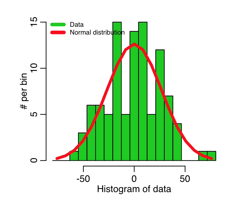
Recall that this fit was to simulated data, that we simulated with a homoskedastic Normal distribution for each point, with std deviation equal to 25.
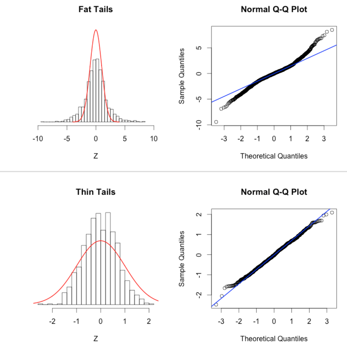
Another diagnostic for Normality is a quantile-quantile (qq plot). It plots the Normalized data (data minus its mean, and divided by its std deviation) versus the expected Normal std deviation for that point, given its rank value. So, for example, if we have 100 data points, the rank of the minimum value is 1, and the rank of the maximum value is 100. We would expect the Normal deviation for that minimum value to be qnorm(1/100)=-2.37. The expected Normal deviation for the next highest value would be qnorm(2/100)=-2.05, and so on (in reality, in the qq plot we actually calculate the expected deviation using qnorm((rank-0.5)/N) where N is the size of the sample). The following code does this, and overlays the expected 45 degree line on the plot (the line the data would ideally follow if it were Normally distributed):
x = myfit$residuals
qqnorm((x-mean(x))/sd(x),cex=1.5,ylab="Normalized data values",xlab="Expected value for Normal data",pch=20)
qqline((x-mean(x))/sd(x),col=3,lwd=2)
which produces the plot
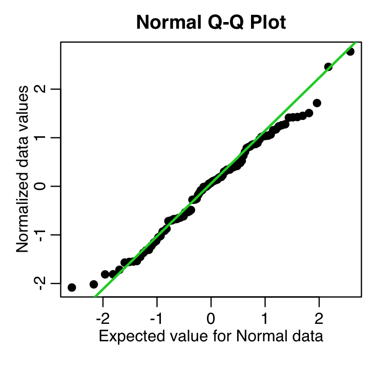
recall that these are residuals from a fit to simulated data that we generated using a Normal distribution. These data should thus follow the green line closely in the qq plot, and they do.
This page describes some qq-plot diagnostics to detect non-Normal data. This page also has nice examples of the pathologies that can lead to non-linear QQ plots: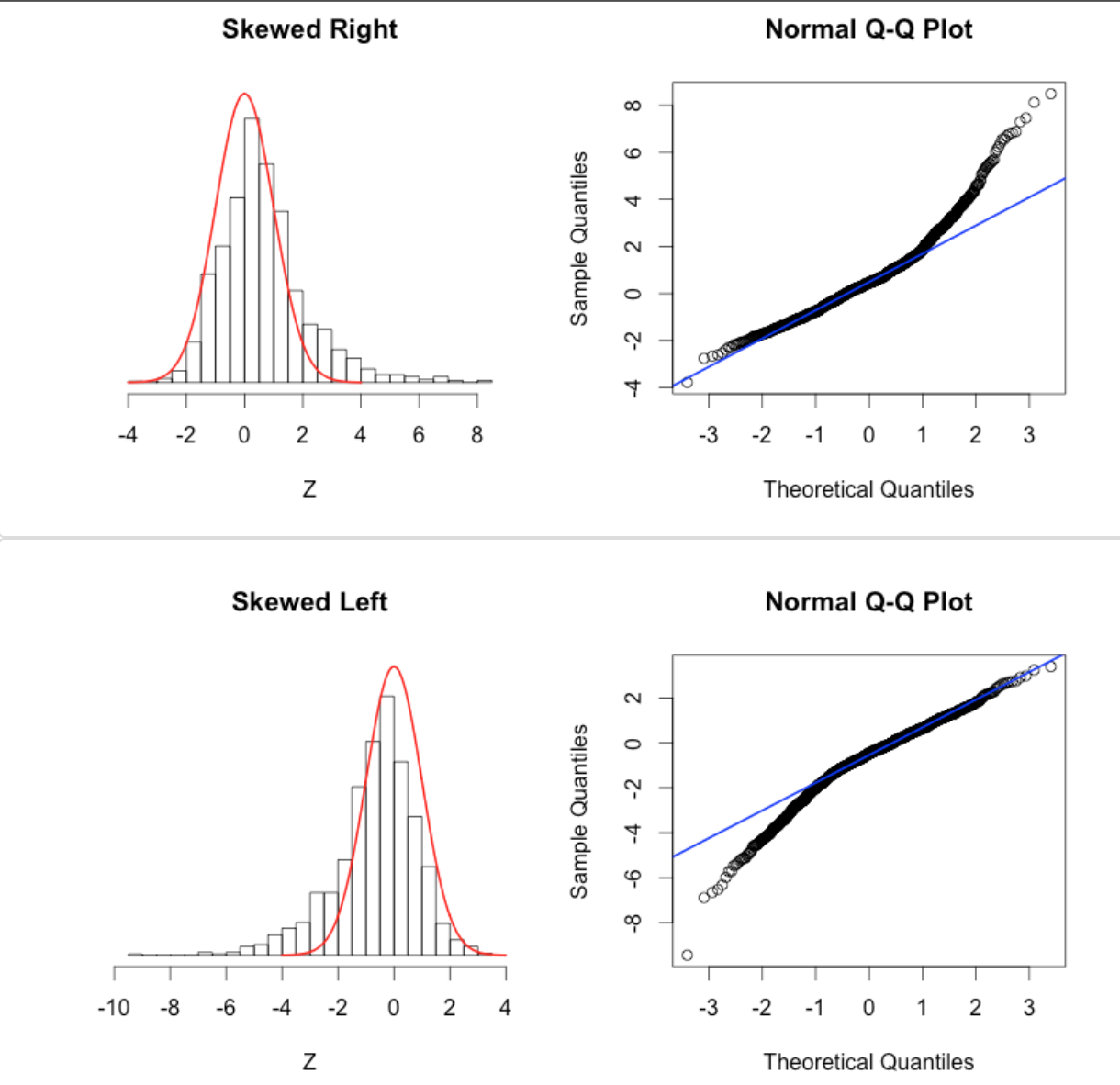
The AML_course_libs.R script also has a method norm_overlay_and_qq() that not only overlays a Normal distribution on the residuals from the fit, but also produces the QQ plot.
The Shapiro-Wilk test can be used to test the null hypothesis that the data are Normally distributed. If the p-value from the test is low, it indicates the data are not statistically consistent with being Normally distributed.
shapiro.test(myfit$residuals)
which produces the output
Shapiro-Wilk normality test
data: myfit$residuals
W = 0.9874, p-value = 0.4654
If you were writing about the results of this test in a paper or your thesis, you would say “the fit residuals were found to be statistically consistent with being Normally distributed (Shapiro-Wilk test p-value p=0.47)”
If there is significant evidence of non-Normality of the residuals, there may be a variety of reasons why, including a confounding variable that might need to be taken into account, or the data may need to be transformed to ensure homoskedasticity. We’ll talk about transformation of data in a later module.
Testing homoskedasticity assumption
In order to test whether or not the data appear to be homoskedastic, it is informative to first make a plot of the fit residuals versus one of the explanatory variables:
plot(mydata$x,myfit$residuals,xlab="X",ylab="Fit residuals",cex=2)
lines(c(-1e6,1e6),c(0,0),col=2,lwd=3)
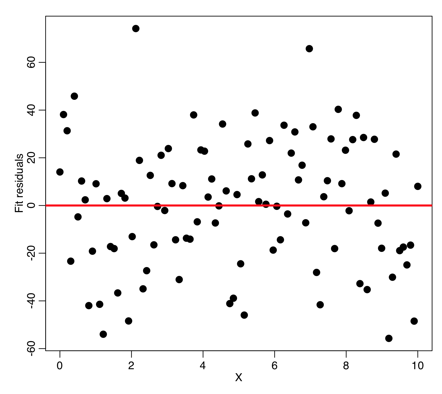
What you’re looking for in a plot like this are points being systematically more closely grouped around zero for some values of the explanatory variable, and systematically more loosely clustered around zero for other values. In this particular case, this doesn’t appear to be evident.
R also has a method ncvTest in the car library that tests a model for heteroskedasticity of the residuals using the Breusch-Pagan test.
install.packages("car")
require("car")
ncvTest(myfit)
The p-value tests the null hypothesis that the data are homoskedastic. The above code produces the output:
Non-constant Variance Score Test
Variance formula: ~ fitted.values
Chisquare = 0.04028789 Df = 1 p = 0.8409187
Parsimonious model selection
You will notice at the bottom of the summary output for our original linear model that it not only gives the R^2, but also something called the adjusted R^2. This takes us to the topic of what happens if you put too many explanatory variables into the model; if, instead of just a linear model, we used a model with a polynomial with degree N-1, we would be able to exactly fit the data (thus R^2 would be exactly equal to 1). However that polynomial, if extrapolated to predict the y at a new value of x, would almost certainly do a very poor job of properly estimating y for another independent, equivalent dataset. This is because that polynomial is likely fitting to the random wiggles of the stochasticity in y in the original data set, rather than representing the true underlying relationship between x and y for that kind of data. The adjusted R^2 penalizes the R^2 statistic to correct for having too many explanatory variables in the model:

From Wikipedia: “If a set of explanatory variables with a predetermined hierarchy of importance are introduced into a regression one at a time, with the adjusted R2 computed each time, the level at which adjusted R2 reaches a maximum, and decreases afterward, would be the regression with the ideal combination of having the best fit without excess/unnecessary terms.”
The principle behind the adjusted R2 statistic can be seen by rewriting the ordinary R2 as
where 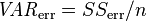 and
and  are the sample variances of the estimated residuals and the dependent variable respectively, which can be seen as biased estimates of the population variances of the errors and of the dependent variable. These estimates are replaced by statistically unbiased versions:
  and
and  .
.
There is also another statistic, called the Akaike Information Criterion (AIC), that can help determine if a model term improves the description of the data while also yielding a parsimonious model; in fact, model selection by minimizing the AIC is the preferred method over maximizing the adjusted R^2. The optimal model minimizes the AIC. There is also another statistic called the Bayesian Information Criterion that does much the same thing.
The R MASS library includes methods related to the AIC. To access the AIC statistic of the linear model we calculated above, install the MASS library, and type
require("MASS")
AIC(b)
For the above simulated data, let’s see if a quadratic model gives us a better adjusted R^2 and/or AIC. Try this:
require("sfsmisc")
set.seed(77134)
n = 100
x = seq(0,10,length=n)
y = 10*x+rnorm(n,0,25)
mydata = data.frame(x,y)

b=lm(y~x+x*x,data=mydata)
print(summary(b))
Is the output what you expected?
It turns out that in R you can’t use powers of x on the RHS. Instead you have to define a new variable, called say, x2, that is x2=x*x, and then put that new variable on the RHS if you want a quadratic term. Or, you could also use the R I() function which tells R to use the terms as specified in the brackets. Try this
mydata$x2=mydata$x^2
ba = lm(y~x,data=mydata)
print(summary(ba))
print(AIC(ba))
b = lm(y~x+x2,data=mydata)
bb = lm(y~x+I(x*x),data=mydata)
print(summary(b))
print(summary(bb))
print(AIC(b))
Is the quadratic term significant? What is the adjusted R^2 and AIC and statistics compared to the model with just the linear term. Does something perhaps seem a little odd?
Now add in a cubic term. What is the significance of the parameters, and what is the adjusted R^2 and AIC statistics compared to the model with just the linear term?
Add in a fourth order term and get the R^2 and AIC statistics and compare them to those of the other models we’ve tried.
We know that the underlying model is linear (because we generated it with y=10*x plus stochasticity). And yet, just based on adjusted R^2 and the AIC statistics, a model with higher order polynomials appears to be preferred. What is going on here?
It turns out that even just looking at the adjusted R^2 and/or the significance of the model parameters does not necessarily give the best indication of the most parsimonious model. The problem is that the stochasticity in the data can make the data appear to be consistent with a different model than the true underlying model. A model that is tuned to the stochasticity in the data may have poor predictive power for predicting future events.
Determination of whether or not our fitted model has good predictive power for future events brings us to the topic of model validation.
Model validation
Model validation ensures that a hypothesized model whose models are fit to a particular data set has good predictive power for a similar data set. A good way to validate a model is a method called “bootstrapping” or “cross-validation”; for example, we could randomly divide the data into half, fit the model on one half (the training sample), then evaluate how much of the variance of the other half (the testing sample) is described by the predictions from the fitted model. A model with good predictive power will describe much of the variance in the testing sample.
The R script least_square_example.R gives an example of bootstrapping by randomly dividing a data set in half to compare the predictive performance of a linear and a quadratic model on the data set we generated above.
Bootstrapping methods also include randomly selecting training and testing samples of the same size of the data from the data, but with replacement. If we were randomly selecting with replacement a set of N numbered balls from a bag, this means that once we select a ball and record its number, we put it back into the bag. Thus, if we do this selection N times, some balls will likely be missed, and some balls will likely be selected two or more times.
More on parsimonious model selection
As discussed, we wish to obtain the most parsimonious model that describes as much of the variance in the data as possible. If we have several explanatory variables that we believe the data might be related to, what we could do is try all different combinations of the variables, and pick the model with the smallest AIC (and check using model validation to ensure that model has good predictive power). However, if there are a lot of variables this procedure would rapidly become quite tedious. The MASS library in R conveniently has a function called stepAIC() that can do this for you. The stepAIC function has an option called “direction”. If direction=”backward”, then the algorithm starts with the model with all variables, and drops them one at a time, picking the model that has the lowest AIC (I believe it drops them in the reverse order as you write them in the model expression in the lm() function). It stops when dropping more terms results in a model with a higher AIC. If direction=”forward”, then it starts with the first variable, and adds the other variables one at a time until the model with the lowest AIC is reached. If direction=”both”, then it essentially adds and drops parameters at each step to determine the model with the lowest AIC. This last option is the preferable one, but can be computationally intensive if your model has a lot of potential explanatory variables.
As an example, let’s assume that we think daily average temperature and wind speed might affect the number of assults per day in Chicago (perhaps by making people more irritable when the weather is bad). Let’s use this code to try out a model with these explanatory variables (you first need to download the files chicago_crime_summary_b.csv and chicago_weather_summary.csv to your working directory, if you have not done so already):
require("sfsmisc")
require("chron")
cdat = read.table("chicago_crime_summary_b.csv",header=T,sep=",",as.is=T)
cdat$jul = julian(cdat$month,cdat$day,cdat$year)
names(cdat)[which(names(cdat)=="julian")] = "jul"
wdat = read.table("chicago_weather_summary.csv",header=T,sep=",",as.is=T)
wdat$jul = julian(wdat$month,wdat$day,wdat$year)

###################################################################
# subset the samples such that they cover the same time period
###################################################################
wdat=subset(wdat,jul%in%cdat$jul)
cdat=subset(cdat,jul%in%wdat$jul)

###################################################################
# put temperature and wind info in the crime data frame
###################################################################
cdat$temperature[match(wdat$jul,cdat$jul)] = wdat$temperature
cdat$wind[match(wdat$jul,cdat$jul)] = wdat$wind

###################################################################
# regress the number of assaults (x4) on daily avg
# temperature and wind
###################################################################
mult.fig(1,main="Number daily assaults in Chicago, 2001 to 2012")
b = lm(x4~temperature+wind,data=cdat)
plot(cdat$jul,cdat$x4,xlab="Julian days",ylab="\043 assaults/day")
lines(cdat$jul,b$fitted.values,col=2,lwd=4)
The code produces the following plot: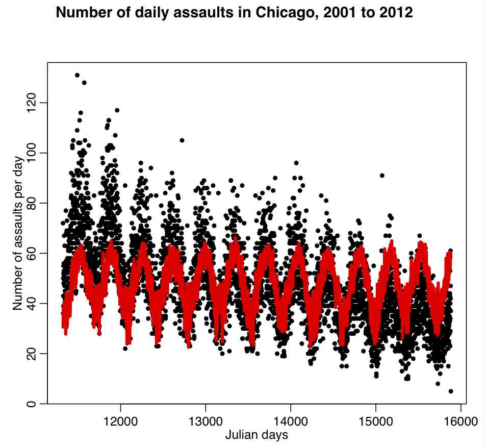
Do you see a problem with this fit?
Try the following code:
mult.fig(1,main="Number of daily assaults in Chicago, 2001-2012")
cdat$jul2 = cdat$jul^2
bb = lm(x4~jul+jul2+temperature+wind,data=cdat)
plot(cdat$jul,cdat$x4,xlab="Julian days",ylab="\043 assaults/day")
lines(cdat$jul,bb$fitted.values,col=2,lwd=4)
It produces the following plot:
What do you think of this fit, based on the figure?
From the fit output, does it look like wind is needed in the fit? Try using newfit=stepAIC(bb,direction=”both”) to determine what the most parsimonious model based on these explanatory variables is. What is the AIC of the original model, bb? What is the AIC of the newfit model? How much of the variance did the model in bb explain? How much of the variance did the model in newfit explain?
As an aside, what kind of possible confounding variables do you think we probably should think about including in the regression?
Also, as an aside, do you think the data are consistent with the underlying assumptions of Least Squares regression? (hint: start by plotting the residuals vs time. Also, there is the norm_overlay_and_qq() function in AML_course_libs.R that can help you figure out if the data are consistent with the underlying assumptions of the statistical model).
Factor regression
In regression analysis we can take into account the effect of what are known as categorical or factor variables; that is to say variables that can take on a variety of nominal levels. Examples of categorical variables are gender, day-of-week, month-of-year, political party, state, etc. An example of factor regression is regressing income on number of years in school, taking into account gender: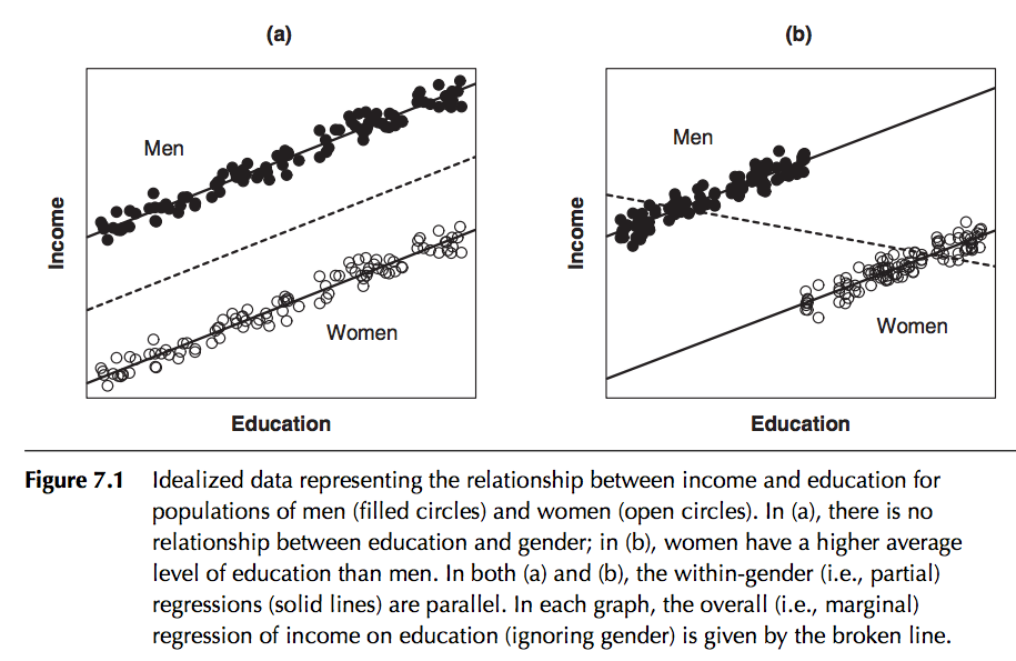
In this particular example, the slope is assumed to be the same for both genders, but the intercept is different. Is it obvious that in this case including gender in the regression will dramatically reduce the residual variance of the model? (ie; increase the R^2)
This is an example of one way to include factor variables in a linear regression fit; assume that for each category the intercept of the regression line is different in the different categories. As we will see in a minute, if we use the lm() function for factor regression, by default R picks one of the categories as the “baseline” category, and then quotes an intercept relative to this baseline for each of the other categories.
Let’s look at an example: let’s assume that the number of assaults in Chicago per day is related to a continuous explanatory variable x that is not a factor (say, temperature), and another explanatory variable w that is categorical (say, weekday). To understand this better, let’s first fit a regression model with just temperature (plus a quadratic trend term in time), then aggregate the residuals by weekday. Is it clear that if there is in fact no dependence on weekday, the residuals within-weekday should be statistically consistent with each other?
The following R code performs the fit and aggregates the results within weekday:
cdat$jul2 = cdat$jul^2
b = lm(x4~jul+jul2+temperature,data=cdat)
plot(cdat$jul,cdat$x4)
lines(cdat$jul,b$fitted.values,col=2,lwd=3)
g = aggregate(b$residuals,by=list(cdat$weekday),FUN="mean")
eg = aggregate(b$residuals,by=list(cdat$weekday),FUN="se")
glen = aggregate(b$residuals,by=list(cdat$weekday),FUN="length")
As an aside: here I used a quadratic term to take into account long-term trends. Do you think higher order polynomials should be used? How could we tell? If we are trying to determine what explanatory variables like temperature may cause crime trends, what is the danger of adding in too many higher order terms in the trend polynomial?
In the file AML_course_libs.R I have included a function called factorplot() that takes a vector y and its uncertainties ey, and plots them along with with mean of y and its one standard deviation uncertainties
source("AML_course_libs.R")
y = g[[2]]
ey = eg[[2]]
ylen = glen[[2]]
factorplot(y,ey)
The code produces the following plot: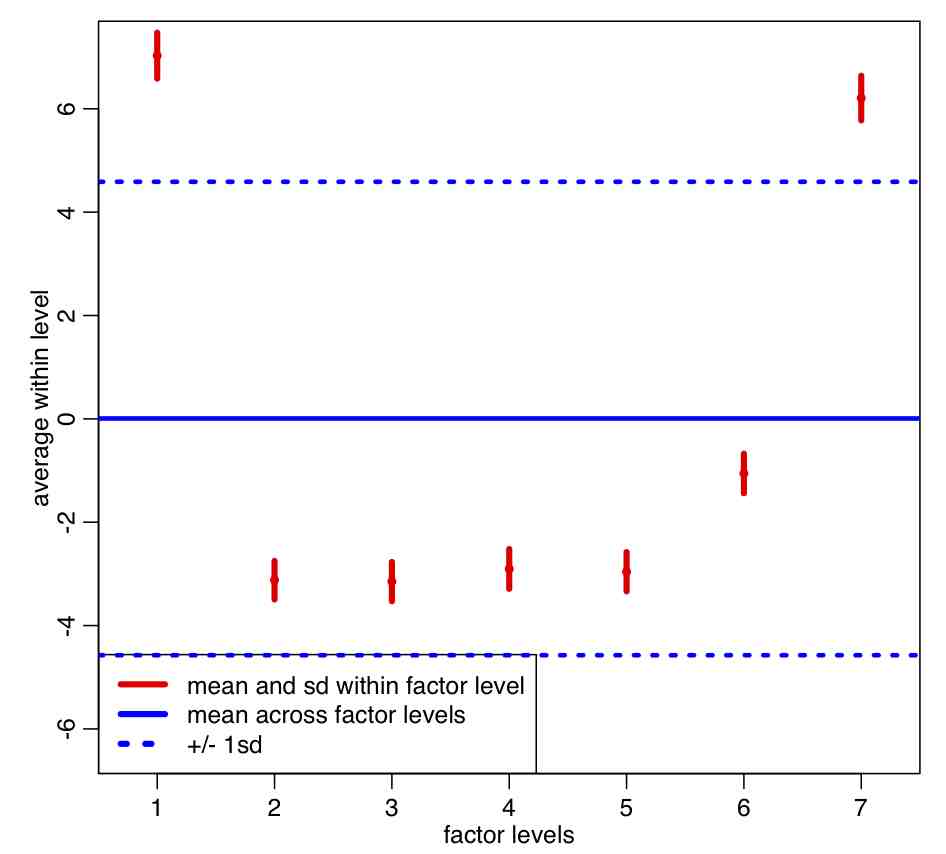
Note that the within-group sample standard deviation (red error bars) is a lot smaller than the pooled standard deviation (blue dotted lines) . Based on the plot, do you think the means of residuals within weekday appear to be statistically consistent?
Let’s test the p-value of that null hypothesis using the chi-square test:
v = (y-mean(y))/ey
dof = length(v)-1
p = 1-pchisq(sum(v^2),dof)
cat("The p-value testing the null-hypothesis that the factor levels are drawn from the same mean is",p,"\n")
Now let’s include the weekday factor level in the regression itself. First let’s fill the weekday name in cdat (recall that weekday=0 is Sunday and weekday=6 is Saturday).
vweekday = c("Sunday","Monday","Tuesday","Wednesday","Thursday","Friday","Saturday")
cdat$weekday_name = vweekday[cdat$weekday+1]
In order to include a factor in the linear regression with lm(), you simply add a term in the call function using factor(<variable name>). R then picks one of the levels of that factor as the “baseline” level (the baseline also includes the overall intercept of the model), and it gives the intercept for the other levels relative to that baseline:
myfit = lm(x4~jul+jul2+temperature+factor(weekday_name),data=cdat)
print(summary(myfit))
Take a look at the output… notice that R picked “Friday” as the baseline. Why do you think that is?
To force R to put the factors in a particular order such that the first in the list is treated as the baseline, you would do the following:
vweekday = c("Sunday","Monday","Tuesday","Wednesday","Thursday","Friday","Saturday")
myfit = lm(x4~jul+jul2+temperature+factor(weekday_name,levels=vweekday),data=cdat)
print(summary(myfit))
Now, take a look at the intercept for Monday, and subtract it from Tuesday. Compare this to y[3]-y[2] from the y vector that we calculated above from the fit residuals within-weekday of the regression model with just temperature and the quadratic trend term. What do you notice?
Interpretation of the summary(myfit) output reveals that all of the factor levels are significant when compared to the Sunday level.
Including interaction terms
In the above we examined adding in higher order polynomial terms of one explanatory variable into the model. If you believe that there are interaction terms between the explanatory variables you can easily include them in a model. Let’s start with a simple example of a drug treatment trial with men and women, and they measured some response vs dosage (for instance, perhaps cholesterol level if it is a cholesterol reducing drug). It is not uncommon for men and women to metabolize drugs differently.
In the trial, 90 men and 90 women are recruited who had high cholesterol. They were divided into groups of 10, and each group was given a different dosage of a drug, and the response in their cholesterol level evaluated after a period of time. The data are in the file drug_treatment.csv Read in this file, and regress the response on the drug dosage without taking into account gender:
ddat=read.table("drug_treatment.csv",header=T,sep=",",as.is=T)
b = lm(cholesterol~dosage,data=ddat)
par(mfrow=c(1,1))
plot(ddat$dosage,ddat$cholesterol,xlab="Drug dosage (mg)",ylab="Cholesterol (mg/dL)")
lines(ddat$dosage,b$fitted.values,col=2,lwd=5)
This produces the following plot.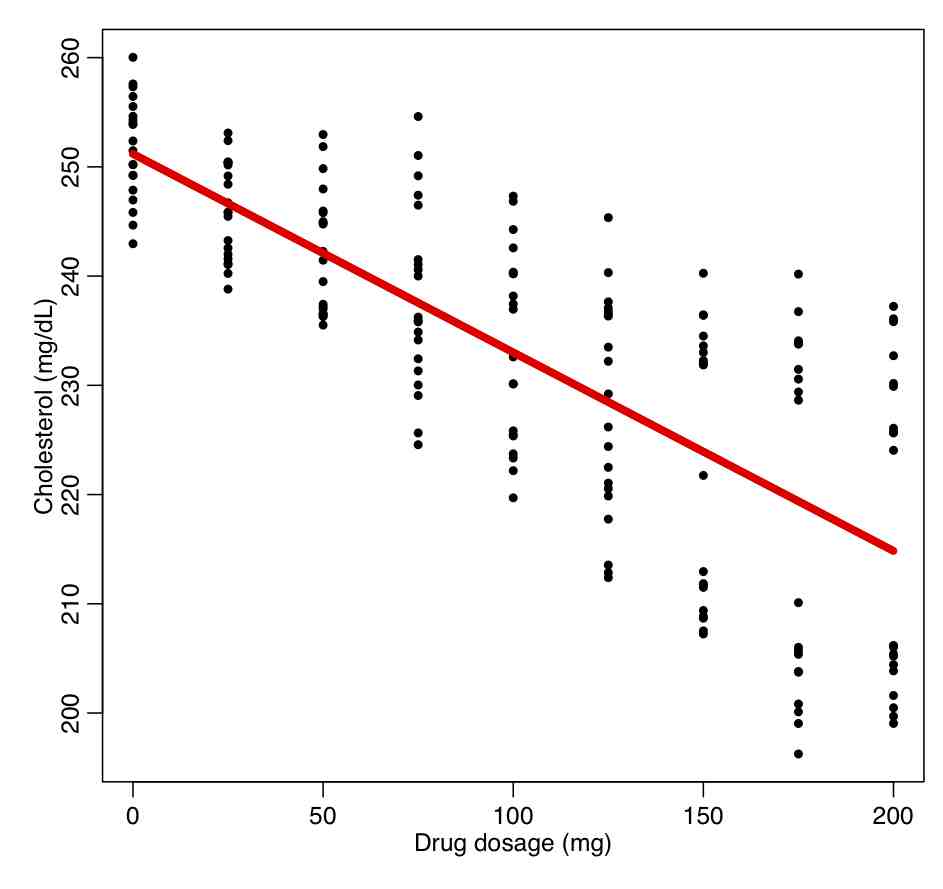
What do you think about the quality of the fit? Are the fit residuals consistent with being Normally distributed? (plot them vs dosage, and also see the norm_overlay_and_qq() function in AML_course_libs.R).
mult.fig(4)
plot(ddat$dosage,b$residuals,xlab="Drug dosage (mg)",ylab="Fit residuals")
source("AML_course_libs.R")
norm_overlay_and_qq(b$residuals)
Now let’s include gender as a factor:
bb = lm(cholesterol~dosage+factor(gender),data=ddat)
par(mfrow=c(1,1))
plot(ddat$dosage,ddat$cholesterol,xlab="Drug dosage (mg)",ylab="Cholesterol (mg/dL)")
for (igender in levels(ddat$gender)){
lines(ddat$dosage[ddat$gender==igender],bb$fitted.values[ddat$gender==igender],col=2,lwd=5)
}
producing this plot: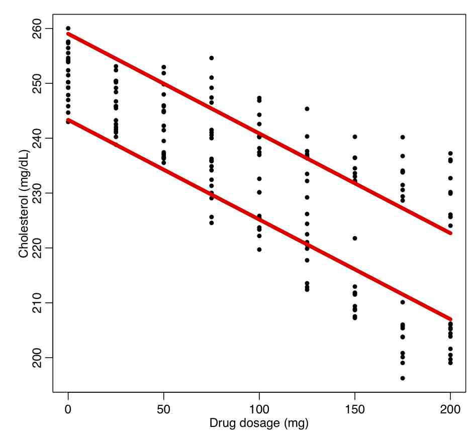
What do you think about the quality of this fit? What is the R^2 compared to the original fit? Do the factor terms appear to be significant? Interpret the results as shown in summary(bb). What is the AIC compared to the original fit? Do the residuals satisfy the underlying assumptions of the Least Squares model?
You can also include interaction terms in a factor regression model if you think that the slope of the regression on the continuous explanatory variable depends on the factor level. In R you do this by multiplying the factor by the continuous variable:
bc = lm(cholesterol~dosage*factor(gender),data=ddat)
summary(bc)
par(mfrow=c(1,1))
plot(ddat$dosage,ddat$cholesterol,xlab="Drug dosage (mg)",ylab="Cholesterol (mg/dL)")
for (igender in levels(ddat$gender)){
lines(ddat$dosage[ddat$gender==igender],bc$fitted.values[ddat$gender==igender],col=2,lwd=5)
}
This produces the plot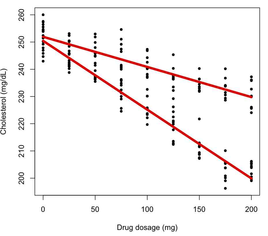
and the fit summary information:
Coefficients:
Estimate Std. Error t value Pr(>|t|)
(Intercept) 250.442396 0.818672 305.913 <2e-16 ***
dosage -0.252715 0.006878 -36.741 <2e-16 ***
factor(gender)M 1.487949 1.157777 1.285 0.2
dosage:factor(gender)M 0.141957 0.009727 14.594 <2e-16 ***
The first term is the intercept for the first factor level (females). The second term is slope for the first factor level. The third term is the difference in intercept for the males compared to the females. The fourth term is the difference in slope for the males compared to the slope for the females. What is the interpretation of the third term not being significant?
Examine the residuals. Are the consistent with the underlying assumptions of the Least Squares method?
Try doing separate regressions with each factor level:
ddat_female = subset(ddat,gender=="F")
bc_female = lm(cholesterol~dosage,data=ddat_female)
cat("Female regression:\n")
print(summary(bc_female))

ddat_male = subset(ddat,gender=="M")
bc_male = lm(cholesterol~dosage,data=ddat_male)
cat("Male regression:\n")
print(summary(bc_male))
with output:
Female regression:
(Intercept) 250.442396 0.808410 309.80 <2e-16 ***
dosage -0.252715 0.006792 -37.21 <2e-16 ***

Male regression:
(Intercept) 251.930344 0.828807 303.97 <2e-16 ***
dosage -0.110758 0.006963 -15.91 <2e-16 ***
Compare the differences, and uncertainties on the differences, of the slope and intercepts from the two fits the results of the combined fit with interaction term above. What do you find?
Use the stepAIC() function in the MASS library on the model bc above. What do you find?
If we wanted to fix the intercept to be the same for the factor levels, but only include different slopes for each factor level, we would do the following:
bd = lm(cholesterol~dosage:factor(gender),data=ddat)
print(summary(bd))
par(mfrow=c(1,1))
plot(ddat$dosage,ddat$cholesterol,xlab="Drug dosage (mg)",ylab="Cholesterol (mg/dL)")
for (igender in levels(ddat$gender)){
lines(ddat$dosage[ddat$gender==igender],bd$fitted.values[ddat$gender==igender],col=2,lwd=5)
}
producing the following plot: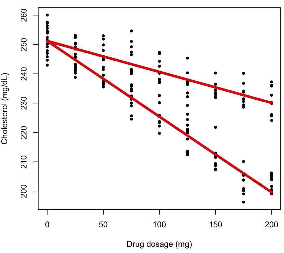
You can also include interaction terms between continuous explanatory variables. For instance, in the below code, we fit simulated data generated with the model y = 50*x*w:
set.seed(89235)
n = 100000
x = rnorm(n,10,0.1)
w = rnorm(n,10,0.25)

y = 50*x*w + rnorm(n,0,25)

myfit_a = lm(y~x+w)
mult.fig(1,main="True model y=50xw")
plot(x*w,myfit_a$residuals,xlab="x*w",ylab="Residuals from fit of y=x+w model")

myfit_b = lm(y~x*w)
summary(myfit_a)
summary(myfit_b)
AIC(myfit_a)
AIC(myfit_b)
Notice that in the first fit we just fit the additive model with no interactions, and it appears to describe a large amount of the variance in the data, even though it is not the correct model. Notice that, unlike with the factor regression for assualts as a function of weekday example given above, plotting the residuals of this additive model fit vs x*w doesn’t seem to reveal any dependence on x*w: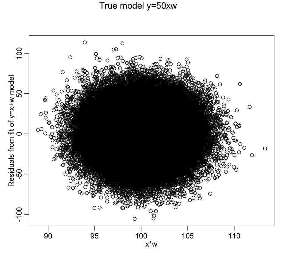
There is no apparent dependence of the linear fit residuals on the interaction term because coefficients of the linear terms mostly compensated for the fact the fit was missing the x:w component. So, just plotting the residuals of an additive model vs cross terms will not usually give an indication as to whether cross-terms may be needed in the fit.
That being said, just like as for any other variable, putting cross-term variables willy nilly into a fit for no well-motivated reason is a bad idea, because sometimes, just due to stochasticity in the data, the cross-term will appear to be significant, and the AIC will make it appear that the term should be in the fit, when it in fact really isn’t related to variation in the dependent variable. This affects the prediction accuracy of the model.
In the myfit_b fit we take into account the cross-terms. Are the regression parameter estimates consistent with what we expect? Is this more complex model preferred?