Most journals in the field of mathematical epidemiology/biology require that you submit manuscripts in LaTeX format.

LaTeX is a word processing language, in which you create a document that contains directives to the latex compiler to produce a final document.  LaTeX provides many capabilities not available in Word; perhaps most important to mathematicians, LaTeX enables typesetting of complex equations that would be difficult, if not impossible in Word.

In addition, LaTeX has a reference management package called BibTeX that easily enables citation of references within your document.

In this module, we will discuss some simple examples of document formatting in LaTeX, and describe how to include figures and tables in the document, and cite references.

There are lots of websites that provide introductions to LaTeX.  For instance, here and here.  In this module I provide a template file that can help to get you quickly started using LaTeX to describe an analysis in mathematical epidemiology/biology.

The file latex_example.tex is a fairly simple template of a LaTeX article document, which might represent the beginnings of an unfinished paper on the use of a mathematical contagion model to simulate the spread of popular memes on the Internet.

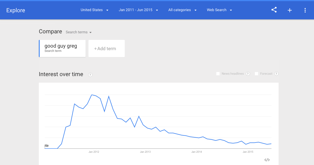
An example of a meme discussed in the paper is Good Guy Greg:

(I’ve got to admit that I have no idea with the one on the upper right means…)

Using Google Trends, we can get the time series of Internet searches related to Good Guy Greg (presumably because someone saw the meme on social media, or was looking to a meme generator to generate their own, etc).  We can hypothetically use the Internet search activity as a proxy for how often the meme is being used over time, and include the plots of the screenshots in our paper:

 

In order to compile the file latex_example.tex, you will also need the figure in encapsulated postscript format, figure_latex_example.eps, which you can find here.  You will also need the BibTeX .bib file, latex_example.bib, which you can find here.  You will notice that in the latex_example.bib file I have annotated many of the bibliographic entries in the file with things like the abstract of the paper. Also note that there are more references in that file than are cited in the paper; you can put as many entries as you want in a .bib file… you don’t need to cite them all.  The latex_example.bib file is just a simple example I came up with for this module.  For an example of a real bibtex file I’ve actually used in my research (with much more extensive annotations in the bibliography) see real_example.bib.  You’ll note that I took pains in that file to carefully annotate all the entries.

Notice that there are a bunch of strange looking lines at the beginning of the latex_example.tex document that are preceded by a backslash, \.  Those are directives to the LaTeX compiler (note that comments in LaTeX are preceded by a % character).  The actual text of the document is contained between the \begin{document} and \end{document} lines.  You’ll notice that I separate blocks of text in the paper using long lines of % characters; I find this helps to make it easier to read.

Also notice that I have my file divided up into the expected sections of a scientific paper (Introduction, Methods, Results, etc), using the LaTeX \section{} directive (commands to the LaTeX compiler are always preceded by a backslash).  LaTex will keep track of the number of sections you have created in your paper, and number them accordingly.  If you want a section of text with a section title, but no number (like, for instance, the Abstract), use the \section*{} directive.

The document includes a figure. Notice that I provided a descriptive caption for the figure.  In your papers, your figures and tables should be a large part of the narrative of your analysis. As such, they should be as much as possible a stand-alone statement.  Thus, if there are model parameters referred to in the figure, give a brief explanation of what they are.  Otherwise the poor reader, who isn’t as familiar with your model parameters as you are, will have to flip through the paper looking for the parameter definitions.  Many first time readers of your paper will read the Abstract and Introduction, then flip to the figures and tables.

If you have a figure in pdf, png, gif, jpeg, etc format, you will need to convert it to encapsulated postscript in order to include it in your document.  To do that, I often use the services of this website.

Note the many $ characters bracketing expressions in the LaTeX file… those are expressions in mathematics mode.  Math mode uses a special italicized font to distinguish math variables from regular text.  It also allows for special LaTeX directives (which are preceded by a backward slash) which tell the LaTeX compiler to put special symbols, like greek letters, the summation symbol, etc.  Here is a list of various LaTeX special symbols in math mode.

To write more complicated mathematical equations, \begin{eqnarray} and \end{eqnarray} is used.  If it is a multiline set of mathematical equations, \\ is used as a line break.  The &=& formats the equations such that the equal signs all line up.  You will find an example in the file of how to format systems of ODE’s for a compartmental model.

I also give an example of a table in the file, and an example of making a formatted list.

To compile the file from a Linux or Unix machine or a Mac from the terminal (otherwise use LaTex compilation software… there are various products available for Windows and Mac machines that allow you to compile and process LaTeX files to produce pdf documents),  type

latex latex_example
bibtex latex_example
latex latex_example
latex latex_example
dvipdf latex_example

The output will be a file called latex_example.pdf.

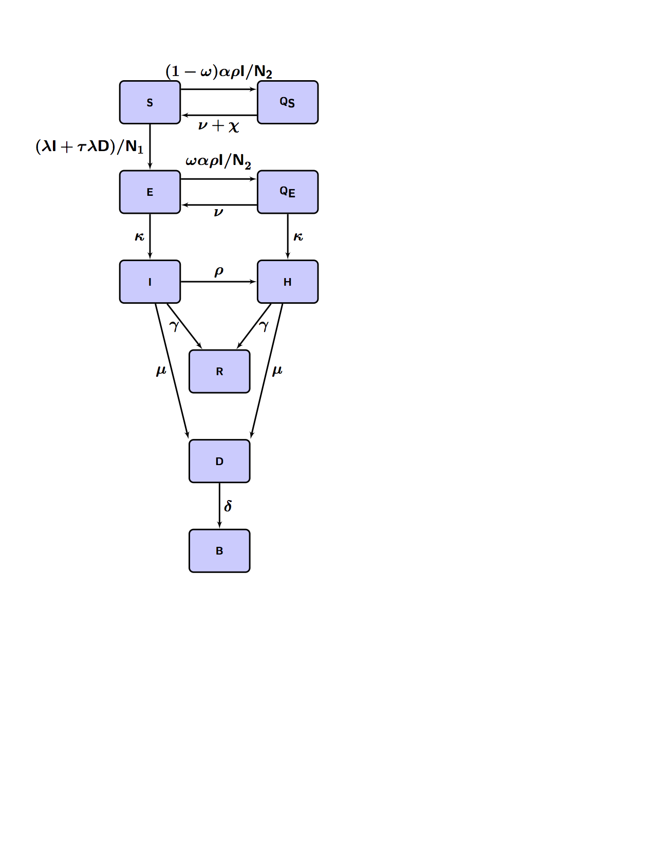
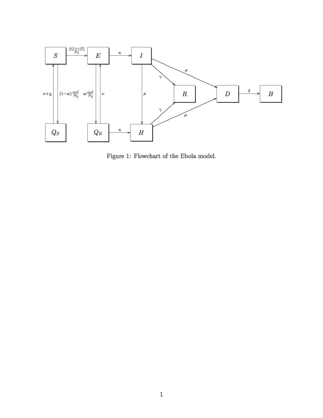
For inclusion of compartmental flow diagrams in LaTeX, you can do one of two things; you can use a graphics program like Paint, Gimp, XFig, etc to create the diagram, convert it to eps, and include it in the document as a figure.  Or, you can actually write the directives within LaTeX itself to create the diagram.

The file example_diagram.tex shows how you can use LaTeX to format a compartmental flow diagram. If you download it to your working directory and type (if you are using Linux or a Mac… otherwise download the file and use your LaTeX processing package to produce the pdf)

latex example_diagram 
dvipdf example_diagram

it produces the pdf file with the following diagram:

There are add-on packages like TikZ that make doing this a lot less inscrutable.  First you need to download the package from the sourceforge website. The file example_diagram_tikz.tex gives an example of how to use methods in the TikZ package.  Download the file to your working directory, and type (if you are using Linux or a Mac)

latex example_diagram_tikz 
dvipdf example_diagram_tikz

This produces the pdf of the same compartmental flow diagram, but a bit nicer looking: