[In this module we will discuss estimates of sample mean and variance, and also discuss the definition of covariance and correlation between two sets of random variables]
Sample moments
Statistics like the sample mean, variance, skewness, and kurtosis are intimately related to the moments of a sample. If we have a sample of n random numbers, X_i, where i=1,…,n, the k^th moment of the sample is
Sample mean
The mean (or average), mu, of the sample is the first moment:
You will also see this notation sometimes
In R, the mean() function returns the average of a vector.
The R script plot_batteries.R reads in the data in trend_corrected_chicago_batteries_2002_to_2013.csv The data include the number of daily batteries (assaults that don’t involve a deadly weapon) in the City of Chicago between 2002 to 2013, along with daily temperature data from Midway airport, daily ozone data from the EPA, and number of daylight hours from NASA. (note that I have done some pre-processing where I trend-corrected the number of batteries, and removed February 29th in leap years, such that the day-of-year variable is always between 1 to 365… also I define a “day” to be from 5am to 4:59 am, because, for instance, 1am Sunday morning is usually considered part of Saturday night).
The plot_batteries.R script reads in this data and calculates the mean of the daily number of batteries, temperature, and daylight hours. It used the very useful R function aggregate() to get the average number of crimes by day of year, and the average temperature by day of year. The aggregate() function has an option by=list(<variable name>). The variable name is the variable within which you would like the data aggregated. Note that this variable needs to be discrete (ie; something like a day, month, year, gender, colour, etc). You can list more than one variable name to aggregate within, btw… here I used just day, but I could have aggregated within year and within month, using the option by=list(year,month).
The aggregate() function also has another option FUN=”<function name>”. If the function name is “mean” then the data are averaged within the variable levels. If the function is “sum” then the data are summed within the variable levels. If the function is “min”/”max” you will get the minimum/maximum within variable levels.
The script also gives a nice example of how to overlay plots of two entirely different quantities on the same plot, with the scale for one on the left hand axis, and the scale for the other on the right hand axis.
The R script produces the plot that shows the means of the various quantities by day of year (note that the script uses the useful R readline(prompt=) function to pause output between plots):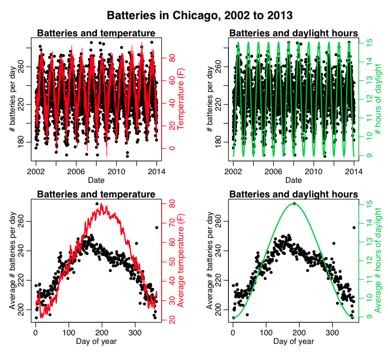
What do you think those big spikes in batteries are at various times of the year? Also, what do you think that more diffuse spike is around day 75-ish of the year?
(I have a theory of crime that I call the Dr. Towers Drunk ‘n Stupid Theory of Crime® that describes many of these fluctuations).
Variance
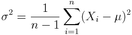
The variance, sigma^2, is a measure of the width of the distribution. It is defined by
![]()
When the true mean of the distribution is known, the equation above is an unbiased estimator for the variance. However, when the mean must be estimated from the sample, it turns out that an estimate of the variance with less bias is
This is referred to as the “sample variance”. In R, the var( ) function returns the sample variance.
The plot_batteries.R script reads in the Chicago battery data and calculates the variance of the daily number of batteries, temperature, and daylight hours.
Standard deviation
The standard deviation of the sample is just the square root of the variance, sigma. In R, the sd( ) function returns the sample standard deviation. Note that if X has units, both the mean and the standard deviation width of X will have those units.
As an aside, you can also use the R sd function in the aggregate() function as an option via FUN=”sd”. This will give you the standard deviation within each of the variable levels.
The plot_batteries.R script reads in the Chicago battery data and calculates the standard deviation of the daily number of batteries, temperature, and daylight hours. It also produces this plot, that shows the mean, and standard deviation widths overlaid on the distributions:
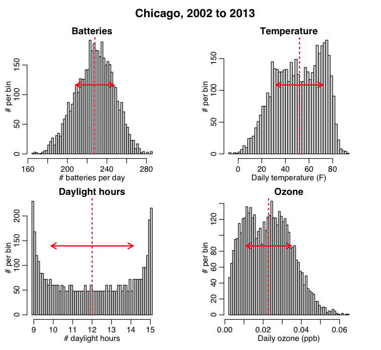
Which of the variables are approximately Normally distributed?
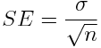
Standard error on the mean
When you estimate the mean of a sample of observations, that is exactly what you are doing… estimating. That estimate may not exactly match the true mean of the probability distribution from which the X are drawn (in fact, it likely won’t). Because the X are random variables, with stochasticity, the estimate of the mean has uncertainty associated with it. The standard error on the mean is the estimate of that uncertainty:
The Central Limit Theorem states that if your sample size is large enough (sample size greater than approximately 25 or so) then, no matter what probability distribution underlies the data, the estimate of the mean will be Normally distributed about the true mean of that probability distribution, with std-dev width of that Normal distribution being equal to SE.
On average 67% of the time the true value of the mean of the underlying probability distribution will lie within the range [mu-SE,mu+SE], where mu is your estimated value. Note that the larger n gets, the smaller SE gets, and the closer your estimated mean will be to the true mean.
Covariance
If we have two samples of the same size, X_i, and Y_i, where i=1,…,n, then the covariance is an estimate of how variation in X is related to variation in Y. The covariance is defined as
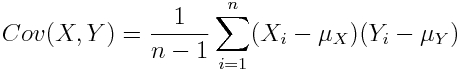
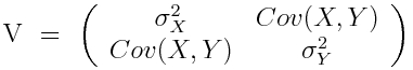
where mu_X is the mean of the X sample, and mu_Y is the mean of the Y sample. Negative covariance means that smaller X tend to be associated with larger Y (and vice versa). Positive covariance means that larger/smaller X are associated with larger/smaller Y. Note that the covariance of X and Y is exactly the same as the covariance of Y and X. Also note that the covariance of X with itself is the variance of X. The covariance matrix for X and Y is thus
The plot_batteries.R script reads in the Chicago battery data and calculates the covariance between the daily number of batteries, temperature, and daylight hours.
Correlation
The covariance has units (units of X times units of Y), and thus it can be difficult to assess how strongly related two quantities are. The correlation coefficient is a dimensionless quantity that helps to assess this.
The correlation coefficient between X and Y normalizes the covariance such that the resulting statistic lies between -1 and 1. The Pearson correlation coefficient is 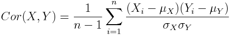
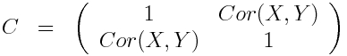
The correlation matrix for X and Y is
The plot_batteries.R script reads in the Chicago battery data and calculates the correlation between the daily number of batteries, and temperature, and daylight hours.
The Fishers Z-transformation can be used to assess whether or not an observed correlation between a sample of N values of X and Y is significantly different than zero.
The Vassar statistics correlation coefficient significance calculator page is a handy online tool for calculating the p-value that tests the null hypothesis that the observed correlation is consistent with zero. The non-directional “two sided test” assesses the probability that we would observe a value of r with absolute value greater than |r_observed| under the null hypothesis that the true correlation underlying the data is zero. The directional “one sided test” assesses the probability that we would observe a value of r at least as large as r_observed (if r_observed is +’ve) under the null hypothesis. If r_observed is negative, it assesses the probability that we would observe a value of r at least as small as r_observed under the null hypothesis that the true r is zero.
Are the observed correlations of the batteries to temperature or daylight hours significantly different than zero? (note that N=4379).
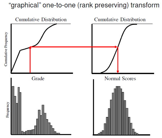
Note that the Fishers Z-transformation significance test assumes that X and Y are Normally distributed. If they aren’t, then applying the test can lead to incorrect p-value assessment. The Spearman rho correlation coefficient helps to fix this, by first mapping the X and Y data onto a Normal distribution using a rank-Normal transformation, then calculating the correlations between the transformed variables. In R, you can obtain the Spearman rho correlation coefficient by using the method=”spearman” option in the cor() method. Here’s how a rank-Normal transformation works (image source):