[In this module, we will describe a simple agent based analogue to a stochastic SIR compartmental disease model]

Agent based modelling methods open up a wide array of possibilities for realistic modelling of biological or social processes.

Unlike compartmental models, with their inherent assumptions of Exponentially distributed compartment sojourn times, agent based models can assume arbitrary probability distributions for state sojourn times.

Nor do the rules for population interactions have to have the full- or partial-homogeneity  mixing assumptions of compartmental models.  With agent based models, you can set up a population with a complex contact network with no randomness whatsoever in the contacts made per day, or a contact network with some randomness, or full homogeneity in the mixing.

In this module, we’ll talk about using agent based modelling methods to simulate the spread of an SIR type disease in a population with homogenous mixing, assuming exponentially distributed sojourn times.  Be aware this is probably one of the most inappropriate implementations of ABM possible… the population is homogeneously mixing and there is no individual level structure in contacts at all! 

Be that as it may…

Setting up an Agent Based model: the state vector

In general, in an agent based model simulating a population of size N, you need to begin by setting up a vector, of length N, that keep tracks of the state each individual currently is in, and (usually) another vector that keeps track of how long they’ve been in that state.  If the population grows or shrinks, so too do the length of these vectors.

You also need to begin with initial conditions for the system (ie; which individual is in what state?).  These are usually randomly assigned.  The R sample(N,x) function will randomly sample x numbers from 1 to N.  Thus sample() can be used to randomly sample the indices of the x individuals who we will label as “infected” in the state vector.

 ##############################################
 # now set up the state vector of the population
 # vstate = 0 means susceptible
 # vstate = 1 means infected
 # vstate = 2 means recovered
 # randomly pick I_0 of the people to be infected
 ##############################################
 vstate = rep(0,N)
 index_inf = sample(N,I_0) # randomly pick I_0 people from N
 vstate[index_inf] = 1 # these are the infected people

And what is the start time? and what are the initial values of the parameters of the model?

Rules for state transitions

You also need to set up the rules for state transitions.  For example, in an SIR model, individuals do not move directly from the S compartment to the R compartment.  They have to transit through the I compartment first.

What has to happen in order for a state transition to occur?  In the case of an SIR model, a susceptible individual only changes state to infectious upon contact with an infectious individual. And by “contact”, we mean “contact sufficient to transmit infection”.

The probability that an infectious person transitions to the recovered state during a particular time step is given by the probability distribution for the sojourn time in that state (and may depend on how long the individual has been in that state).

Infectious individual changing state to recovered state

The sojourn time in the infectious period in a simple SIR model is Exponentially distributed with parameter gamma.  As we described in this previous module, this means that the probability that the individual will recover in time delta_t is

recover_prob=1-exp(-gamma*delta_t)

As gamma*delta_t becomes small, what function does recover_prob approach?

Because the Exponential probability distribution is memoryless, recover_prob is a constant that does not depend on how long the individual has been in the state.  Thus, to determine if the individual recovers during a particular time step, we randomly sample a number, vprob, from Unif(0,1).  If vprob<recover_prob, the individual recovers, and their state changes to “recovered” going into the next time step.

Susceptible individual becoming infected

The rate at which an individual in the S compartment contacts other individuals in the population is beta; thus the average number each individual contacts in time delta_t is delta_t*beta.  We assume in the model that if they “contact” an infected person, the probability of transmission of the pathogen is 100% (thus a “contact” really means “contact sufficient to transmit infection”).  When mixing is homogeneous, a fraction I/N of the people that are contacted will be infectious.  

Thus the average number of infectious people contacted in the population in time delta_t is 

avg_num_infected_people_contacted = delta_t*beta*I/N

But that’s just the average number of infectious people contacted.  The stochasticity in the number of contacts each of the N person makes is Poisson distributed about that average. Thus the number of infectious people contacted at a particular time step by each of the N people is

vpois = rpois(N,avg_num_infected_people_contacted)

If the person is in the susceptible state at the beginning of the time step, and they contacted zero people at that time step, we assume they remain in the susceptible state going into the next time step.  If they contact at least one infectious person, we change their state to infectious.

Doing the simulation

Now that we have our initial conditions, a state vector that keeps track of each individual’s state, and rules for state transitions, the only thing left to set up the simulation is to set a random seed, and loop through the simulation in small steps of time.

The R script sir_agent_func.R shows an example of a function that implements this very simple agent based model.

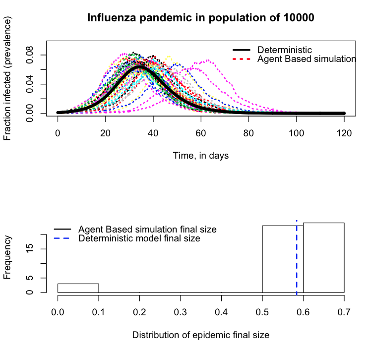
The file sir_agent.R reads in the sir_agent_func.R and implements it to make the following plot by doing 50 realisations of the simulation of a flu like disease circulating in a town of 10,000 individuals.

Making things slightly more complicated: non-Exponentially distributed sojourn times

Exponentially distributed sojourn times have the advantage that we need to keep track of how long the agent has been in a state in order to calculate the probability it will leave it at any particular time step; the probability is always constant due to the memoryless property of the Exponential distribution.

It is usually a quite unrealistic assumption to assume that state sojourn times are exponentially distributed.  In this past post, we discussed how a two parameter “bump-like” distribution like the Gamma distribution can be much more appropriate.  In the post, we also discussed how the linear chain trick could be used with a special form of the Gamma distribution to incorporate non-exponentially distributed sojourn times in a compartmental model.

For example, using the linear chain trick, we can simulate the infectious class sojourn time as being Gamma distributed with shape=k (with integer k), and scale=1/(k*gamma) by expanding the model to have k compartments for the infectious stages, rather than just one.  Like so

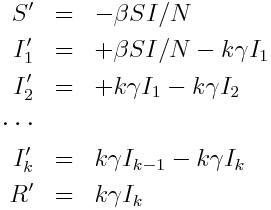
We could, in our agent based model, similarly add in additional compartments to use the linear chain trick to simulate Gamma distributed sojourn times.

Or, we could take a more general approach, that would work with any probability distribution for the sojourn times, where at each time step we calculate the probability that the individual leaves the state based on how long they’ve already been in it, t.

Just like we saw in this post, the probability that the individual leaves a state between [t,t+delta_t] is

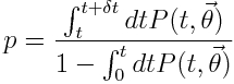
where P(t,vec(theta)) is the probability distribution for the sojourn time, and can depend on the current sojourn time, t, and the model parameters, vec(theta).

For the Gamma distribution with shape=k and scale = 1/(k*gamma), the numerator in the above equation, written in R, is

pgamma(t+delta_t,shape=k,scale=1/(k*gamma))-pgamma(t,shape=k,scale=1/(k*gamma))

To re-iterate, t is not the time since the simulation began, but the time that the individual has been in the state that you need to keep track of to assess the state transition probabilities.  When the individual changes states, t resets to zero and begins incrementing again from thereon forward (either until the simulation ends, or the individual once again changes states).

Notice that because this expression depends on t, we have to keep track of how long individuals have been in a state in order to calculate it.  It’s one more thing to keep track of in an agent based model.

The R script sir_agent_func.R contains a method SIR_agent_erlang() that performs an agent based simultion of an SIR model with homogenous mixing, with Gamma distributed infectious stages.

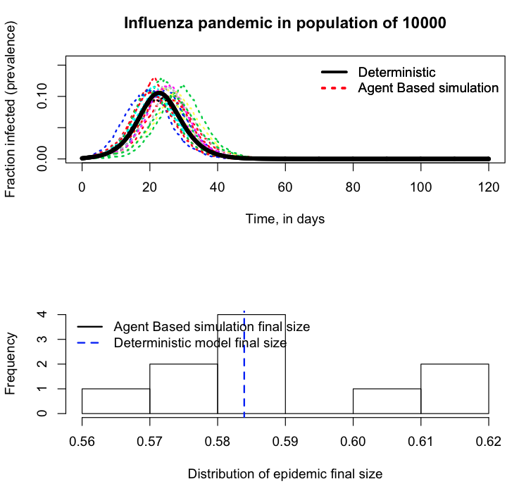
The R script sir_agent_erlang_sojourn.R reads in the sir_agent_func.R file, and runs several realisations of the system for a flu-like disease circulating in a population of 10,000.  The script produces the following plot:

Run this script, and the sir_agent.R script for 10 realisations each.  How much does it slow down the script to have to keep track of the time individuals spend in their state?  Use the R proc.time() function to determine this.