[In the Spring AML612 course at ASU, we have discussed stochastic modelling methods, including Markov Chain Monte Carlo, Stochastic Differential Equations, and agent based models.  Here we discuss how random sampling can contribute stochasticity to observed data]

In past modules, we have discussed how stochasticity in population contact patterns and/or state sojourn times leads to stochasticity in dynamical systems.  For small populations in particular, such stochasticity can lead to wide variation in system outcomes.

However, this is not the only source of stochasticity that may underlie data that we observe for dynamical systems.  For instance, for animal populations, rarely do we count all animals in a population.  Rather, partial counts are done, and inference is made about the overall population size.

With disease, it is very rare to count all cases of infection with a disease.  For instance, it has been estimated for Zika virus infection that 80% of cases are asymptomatic.  And because even the symptomatic cases are usually mild, people don’t go to the doctor.  And even of the people who go to the doctor, the medical center may not participate in an official surveillance system.

For influenza, roughly only one out of every 2 to 5 hospitalizations actually gets officially confirmed by the US surveillance system. And that’s just the hospitalizations (ie; people who are really sick, clearly with some kind of respiratory disease).  Seroprevalence studies estimated that around 20% of the US population was infected with H1N1 during 2009, but only 135,000 cases were actually confirmed by laboratory testing in the surveillance system.  That means that only around 1 on 500 cases were detected by the surveillance system.

Detection by surveillance (or counting of partial populations) involves stochasticity.  If an average fraction, p, of a population of N are randomly sampled, the underlying stochasticity is Binomially distributed as Bin(p,N).  As we are about to see, if p is small, the stochasticity this causes in the data can be much larger than the stochasticity inherent to the dynamical system itself.

An example of how this stochasticity arises: say every person who gets a particular disease gets so ill that they have to see a doctor, and there are N ill people.  However, only one out of 100 doctors in the city participates in a surveillance system.  Each ill person randomly chooses a doctor.  The total number of people seen by the doctors in the surveillance system is Binomially distributed as Bin(p,N).

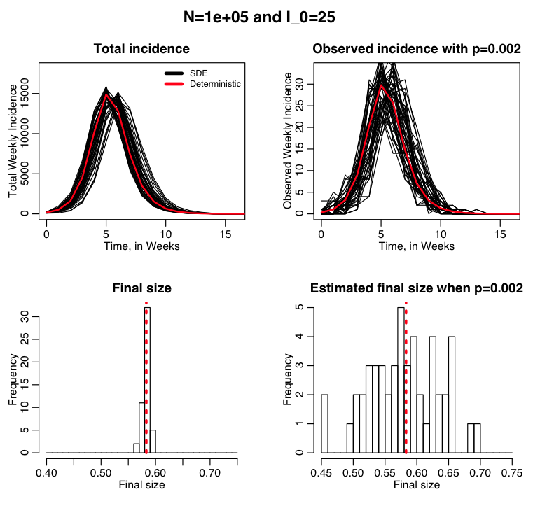
Example: flu like disease spreading in a population of 100,000, with only 1/500 cases detected on average

The R script sir_sde_with_binomial_sampling.R uses stochastic differential equations to simulate the spread of a flu like disease in a modestly sized city of 100,000 people.  We assume that the surveillance system in the city only detects on average 1 out of every 500 cases.  If the public health department in the city knows that on average it detects 1 out over 500 cases, it can infer the total size of the outbreak from the number of cases that they detected.  The script produces the following plot:

Implications of random sampling for independence of data from time point to time point

Early in an outbreak of a newly emerging disease (like Ebola or Zika) one of the first things examined is the exponential rise in cases.  Along with a model, the exponential rise can be used to estimate the basic reproduction number of the disease; the average number of new infections an infectious person causes during the course of their infection in a completely susceptible population.

The fitting methods pretty much universally used to fit an exponential curve to early incidence data assume that the stochasticity in the points are independent from point to point.

What does it mean for data bins to be “independent” in a binned distribution (like, for instance, the time series of the number of newly identified disease cases each week)?  This means that the stochastic variation data in the i^th bin is uncorrelated to the variation in the j^th bin.   Note that the assumption of independent bins underlies the Maximum Likelihood, Least Squares and Pearson chi-squared methods, unless special modification is made to those methods to take the correlations into account.  If you go ahead and use those methods anyway to fit to autocorrelated data, you will get biased fit results, and your confidence intervals on your fit estimates will be wrong.

For Binomial random sampling of data at each time point, the stochasticity from point to point is independent (if you randomly sample slightly lower than average on one day, it has no effect on whether you will sample slightly higher or lower the next).  

However, the additional stochasticity in the system dynamics can result in large autocorrelations in the data (for example, if the number of infectious people fluctuates higher than the deterministic prediction one day, because there are more people now to infect others, subsequent time points in the immediate future will also tend to have higher than average number of infectious people).

But if the Binomial sampling fraction, p, is small, the large relative variations due to Binomial sampling stochasticity from point to point will tend to wash out autocorrelations in the data.

The R script sir_sde_with_binomial_sampling_exponential_rise.R examines the initial exponential rise portion of the epidemic curve of a flu-like illness spreading in a city. It does this for a deterministic model, an SDE model, and an SDE model with additional random Binomial sampling with p=0.01.  The script examines the autocorrelation from point to point of the incidence minus the deterministic prediction for the SDE model, and the SDE model with Binomial random sampling.  The script produces the following plot:

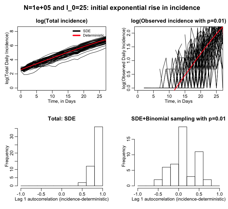
The fluctuations in the SDE model predictions relative to the deterministic model are highly correlated from point to point.  But the fluctuations in the SDE+Binomially sampled model are largely independent from point to point.

Thus, if we fit an exponential curve to observed incidence data with methods like Least Squares or Maximum Likelihood, we can do so with confidence that the stochasticity from point to point is largely independent (which is a relief, because basically every fit to incidence data ever done in the literature assumes the stochasticity is independent from point to point… whew).

The upshot of all of this is that if you are fitting an epidemic model to disease data, or are fitting a population model to population data, if you only partially observe the data the primary stochasticity in that data is likely largely from the randomness of partial observation, not due to the stochasticity in the underlying dynamics of the system.

And so if you expect that your stochastic modelling method will simulate all the stochasticity observed in the data without explicitly adding in additional Binomial stochasticity to account for partial sampling, it won’t.  You might have to add in other major stochastic effects by hand.