
[This module presents a simple introduction to agent based modelling in R of contagion spreading on a network]
The contacts people make in a population can not only be random during a day, as we discussed in this past module, but also determined on a daily basis with more regularity by the people we live with, and go to school or work with. If these contacts remain relatively constant over the course of a disease outbreak, this is an example of a static networked population
When speaking about “contacts” in the context of the spread of disease, what we mean are “contacts sufficient to transmit infection”. We usually think of such contacts between two people as going both ways, having equal probability of spread of contagion upon a contact in either direction. But for some diseases (like HIV, for instance), this isn’t true. For such diseases occurring in a population network, the network is known as a directed graph.
Disease models can be used to simulate the spread of ideas as a contagious process. When talking to your friends and family, the spread of ideas is usually mutual. However, ideas spread on social networks like Facebook and Twitter are a mix of mutual infection, and one-way infection. For instance, the Twitter account of a major news agency follows few other Twitter users, but has many followers. The influence of ideas is mostly uni-directional in that case.
In this module, we’ll examine the spread of a disease on a bi-directional population contact network defined mostly by contacts that occur at home, and work or school.
Grouping people into realistic households requires data on what kinds of households there are, and their relative frequency.
The US Census has kept track of household living arrangements of Americans for many decades. The most recent information on households can be found here.
I’ve downloaded the data set US_household_demographics_2015.csv that has the information regarding the total number of households in the US, the total number of family households. From this information, we can determine the fraction of households that are non family
- A non-family household in the US generally consists of one person living alone.
- A “family” household consists of two or more related people living together. Such households can include couples that do not have kids living at home.
hdat = read.table("US_household_demographics_2015.csv",header=T,sep=",",as.is=T)
hdat[,2] = as.numeric(gsub(",","",hdat[,2]))
nhouse = hdat[89,2]
nnon_family = hdat[99,2]
fnon_family = hdat[99,2]/hdat[89,2]
The US_family_household_characteristics_2015.csv data set has the information on the total number of family households with 0, 1, 2, 3, 4, and 5+ children. The family households with 0 children are couples that do not have kids. From the information in this file, we can determine the probability that a family household has N kids (N=0 to 5+). Nominally, let’s make the simplifying assumption that a household can have at most 5 kids.
udat = read.table("US_family_household_characteristics_2015.csv",header=T,sep=",",as.is=T)
vnum_kids = c(0,1,2,3,4,5)
prob_num_kids = c(udat[97,2],udat[98,2],udat[99,2],udat[100,2],udat[101,2],udat[102,2])
prob_num_kids = as.numeric(gsub(",","",prob_num_kids))
prob_num_kids = prob_num_kids/sum(prob_num_kids)
The US_living_arrangements_of_children_2015.csv data set has information on the number of adults living in households with kids.
cdat = read.table("US_living_arrangements_of_children_2015.csv",header=T,sep=",",as.is=T)
cdat[,2] = as.numeric(gsub(",","",cdat[,2]))
ntot_kid_household = cdat[1,2]
ntot_kid_with_both_parent_household = cdat[4,2]
ftot_kid_with_both_parent_household = cdat[4,2]/cdat[1,2]
When I crunch all the numbers from the three files, here is what I get for the relative fractions of the types of households:
- Non-family households = 0.358
- Family households, 0 kids = 0.3369
- Couple households, 1 kids = 0.0906
- Couple households, 2 kids = 0.0777
- Couple households, 3 kids = 0.0299
- Couple households, 4 kids = 0.0092
- Couple households, 5 kids = 0.0038
- Single-parent households, 1 kids = 0.0403
- Single-parent households, 2 kids = 0.0345
- Single-parent households, 3 kids = 0.0133
- Single-parent households, 4 kids = 0.0041
- Single-parent households, 5 kids = 0.0017
Note that this calculation of relative weights of households assumes that the distribution of children is the same in households headed by a couple compared to single-parent households. In order to get that information, we need cross-tabs, and the Census bureau doesn’t provide the information at that level of detail (at least, as near as I can determine).
Now we need to take our population of Npeople, and assign them to households. The easiest way I’ve found to do this is to assume nothing about their age to begin with, then assign their age (in this case, “kid” or “adult”) once they have been assigned to a household.
Essentially, what we do is randomly draw a type of household out of our bag of households, given the relative weight of each household. We then assign the proper number of people to the household, with ages, and then keep track of the fact that they have connections between each other (via two vectors, named vfrom and vto, for instance, that contain the ID number of the person doing the contacting, and the person being contacted. Because we are assuming our network is bi-directional, both directions of contacts get entered into the vectors. In addition, we can keep track of the expected average number of contacts that would occur between these people per day (let’s call this vector vnavg_contact_per_day)
R code for networking a population into households
The R script pop_structure_utils.R has a function setup_households, that assigns Npeople to households, given household demographics for adults and children.
#############################################################################
# http://www.census.gov/hhes/families/files/cps2015/tabF1-all.csv
# http://www.census.gov/hhes/families/files/cps2015/tabC2-all.csv
# http://www.census.gov/hhes/families/files/cps2015/tabH2-all.csv
#
# assume all "non-family" households consist of one adult
#
# fnon_family Is the number of "non-family" households
# We assume these consist of one adult each
#
# vnum_kids Vector of number of kids in "family" households (goes from 0 to 5)
# "families" can consist of a couple with no kids
#
# prob_num_kids vector of probabilities for observing vnum_kids
#
# ftot_kid_with_both_parent_household Is the fraction of kids living with
# both parents
#############################################################################
setup_households=function(Npeople
                         ,fnon_family
                         ,vnum_kids
                         ,prob_num_kids
                         ,ftot_kid_with_both_parent_household
                         ,navg_contact_per_day)
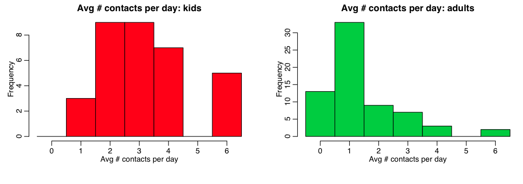
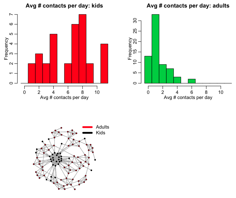
The R script pop_structure.R reads in this file, and uses the setup_household() function to network a population into households. It prints out the fraction of kids in the population (0.33), and also histograms the average number of total daily contacts for kids and adults:
Visualizing a population networked into households
It is informative to visualize the household network structure.
An excellent treatise on network visualisation in R can be found on Katherine Ognyanova’s website.
In order to do network visualization, you first need to install several packages in R
 install.packages("igraph")
 install.packages("network")
 install.packages("sna")
 install.packages("ndtv")
You also need to create a data frame with the ID names of the nodes (let’s call this data frame “nodes”), and another data frame with the links between the nodes (let’s call this data frame “links”). The links data frame will contain the vfrom and vto vectors, and can also contain the average number of contacts expected to be made per day, vnavg_contact_per_day)
 ########################################################################
 ########################################################################
 # create data frames with the node and vertex information
 ########################################################################
 nodes = data.frame(id=vid,col=(vage+1))
 links = data.frame(from=vfrom,to=vto,weight=vnavg_contact_per_day)
 ########################################################################
 # put this information into an igraph network object
 ########################################################################
 net=graph.data.frame(links, nodes, directed=T)
To display the network, we can use the plot() command.
 plot(net
     ,edge.arrow.size=.4
     ,vertex.label=NA
     ,vertex.size=4.0
     ,edge.arrow.size=0.001
     ,edge.arrow.width=0.001
     ,layout=layout,
     ,xlim=c(-1.1,1.1)
     ,ylim=c(-1.1,1.1))
Where layout specifies the graph layout. There are a number that can be used, including putting all the agents on a circle, and connecting them with lines,
layout = layout.circle(net)
which produces a yarn ball, like this:
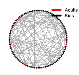
Which is not as visually informative of the underlying network structure as it could be.
Instead, a network graph presentation using something called a force directed algorithm, can yield much more visually informative results.
layout = layout.fruchterman.reingold(a$net, repulserad=vcount(net)^3,area=vcount(net)^2.4)
The R script pop_structure.R uses this to produce the following network graph:

Adding and getting information to and from a network object
The documentation for R methods related to an igraph object can be found online here.
If you have a network object, let’s call it “net”, you can get a list of the edge and vertex attributes of the object by typing
edge.attributes(net)
vertex.attributes(net)
to get the full list, or, if you just want the names of the attributes, type
names(edge.attributes(net))
names(vertex.attributes(net))
Doing this for the network produced in pop_structure.R, yields
> names(edge.attributes(a$net))
   [1] "weight" "vfrom" "vto" "vnavg_contact_per_day"
> names(vertex.attributes(a$net))
   [1] "name" "age" "col" "vid" "vage" "color"
If you take a look at the setup_households() function in pop_structure_utils.R, you will see that I filled many of these network attributes in the script by using commands of the form
 net=graph.data.frame(links, nodes, directed=T)
 V(net)$vid = vid
 V(net)$vage = vage
 E(net)$vfrom = vfrom
 E(net)$vto = vto
 E(net)$vnavg_contact_per_day = vnavg_contact_per_day
 V(net)$color=V(net)$col
Where E(net) sets edge attributes, and V(net) sets vertex attributes.
Setting up school and work contacts
In the pop_structure_utils.R script, there is a function setup_schools_and_workplaces() that further networks a population into school and workplace contacts. It takes as an input an already existing igraph network object, net:
setup_schools_and_workplaces=function(net
                                     ,vn_per_school
                                     ,vnavg_contact_per_day_per_school
                                     ,vn_per_workplace
                                     ,vnavg_contact_per_day_per_workplace
                                     ){
vn_per_school is a vector giving a sample of “school” or “class” sizes that you will randomly apportion the kids into (the function will randomly choose a “class” size to put a group of kids into from this vector). The vnavg_contact_per_day_per_school is the average number of contacts the kids in a class will make during a day.
vn_per_workplace is a vector of “workplace” sizes that you will randomly apportion the adults into. The vnavg_contact_per_day_per_workplace is the average number of contacts per day the adults will make in that workplace.
If linclude_school_and_work = 1 in the pop_structure.R script, the script will network the population into households, and into schools and workplaces. The script produces the plot:
Example of simulating disease spread on a network
The script pop_structure_utils.R has a function that simulates the spread of a Susceptible, Infected, Recovered disease in a networked population, assuming that the infectious period is Exponentially distributed with parameter gamma.
tbeg and tend are the beginning and end time of the simulations, and delta_t is the time step
simulate_sir_disease_spread_on_network=function(net
                                               ,tbeg
                                               ,tend
                                               ,delta_t
                                               ,gamma)
The simulation steps through the time steps, and at each step randomly samples a Poisson distributed number of contacts that each person makes with other people, from the average number of daily contacts expected, times delta_t. If this number is at least one, and the person they contact is infectious (and they are susceptible), the person’s state changes to infectious.
To determine if an infectious person recovers in that time step, we randomly sample a uniform number between 0 and 1. If that number is less than precover=1-exp(-gamma*delta_t), then we assume the person recovers, and we change their state to recovered.
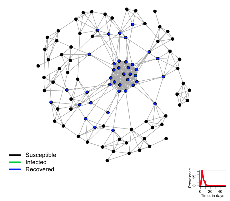
At the beginning of the simulation, the method plots the network, with the nodes coloured according to their state. As the simulation steps through, it colours the nodes according to the current state.
The R script agent_based_sir_on_network.R uses the methods in pop_structure_utils.R to network a population of 100 people, and then simulate the spread of an SIR-type disease on that network. The script produces the following plot, showing the final state of the system (it changes this plot during the simulation, showing the intermediate states of the simulation):
- Try changing the random seed
- What if we change Npeople?
- Try running the simulation with household contacts only (no work or school)
- Try changing the number of contacts at home
- Try changing the number of contacts at work and/or school
- Histogram the number of contacts of kids and adults. What is the average? What is this average divided by gamma?
- How would we go about keeping track of how many infections happened due to home/work/school contacts?