[This module presents Monte Carlo stochastic methods that can be used to assess uncertainty in model estimates due to uncertainty in one or more parameters]

Deterministic mathematical model for dynamical systems, such as the spread of infectious disease, or dynamics in animal populations, involve parameters.  In the case of diseases, these parameters might include things like the incubation and/or infectious periods, and also the transmissibility of the disease.  In the example of animal populations, the parameters might include birth rates, death rates, predation rates, etc.

Many of these parameters are determined from observation.  For instance, Zika, a mosquito borne disease, has been observed to have an incubation period (time to symptoms, and assumed infectiousness) of 3 to 12 days.  That range is derived from examining when people first showed symptoms, relative to an assumed date that they were first exposed (estimated, for instance, by the date that the first of their family members or close contacts showed symptoms).

Obviously, there is not only variation from human to human in the length of the infectious period, but a lot of uncertainty associated with estimating when a contact-sufficient-to-transmit-infection with an infectious person occurred.

The length of the infectious period of a disease is also obtained from observational studies.  And again, there is variation from human to human, but also uncertainty involved in assessing the length of this period.  Is it really the duration of the symptoms?  How clearly demarcated is the beginning and end of symptoms?  And if determined from the viral shedding temporal profile, how much virus needs to be shed to be “infectious”?

For interacting predator/prey populations, predation rates are only estimates (and as such suffer from empirical uncertainties), as are the relative numbers in the populations.

If we would like to use a model to simulate the dynamics of these populations, it is important to realise that parameter uncertainties lead to uncertainties in the model outputs.

Probability distributions underlying parameter uncertainties

Assessing the model output uncertainty requires knowledge of the probability distributions underlying the stochasticity in the parameters.

How the uncertainties on parameters are quoted in the literature can vary quite a bit, and serve to obscure the true underlying probability distribution; many publications will simply quote a range, without indication as to whether or not it is a confidence interval, or just the minimum and maximum values ever observed.  In this case, it is common to assume that the underlying probability distribution is Uniform in that range.

If the range is given as a confidence interval (usually enclosed in square brackets in the form [XX,YY]), unless otherwise specified, the probability distribution underlying the stochasticity is assumed to be Normal.  Why Normal?  Because the parameters are usually estimated from empirical studies with data, and the Central Limit Theorem states that, when the data set is large, the uncertainty on the mean is Normally distributed.

But if the study gives the underlying probability distribution (say, Gamma) you should always assume that probability distribution.

Assessing effect of parameter uncertainties on model predictions

However, even with an estimate of the probability distribution underlying the parameter stochasticity, it is often impossible to obtain analytic expressions for the resulting uncertainty in model estimates.  In the case of disease, this might include the model prediction of final size, for instance, or peak time, or maximum incidence, or endemic equilibrium prevalence, etc.  For animal populations, it might include the prediction for endemic equilibrium sizes of the populations, or maximum or minimum population sizes, etc.

The reason it is often impossible is because analytic expressions often don’t exist for for many of these quantities, which is why we have to do the model numerical simulations in the first place.  Even when such analytic expressions exist for particular model outputs, they are usually very non-linear in the model parameters, and thus it is extraordinarily difficult to get an analytic expression for the resulting probability distribution for the model output of interest.

Stochastic methods for assessing resulting probability distributions on model outputs

The easiest way to assess the probability distribution underlying the model output stochasticity due to parameter uncertainty is to randomly sample values of the parameters from their probability distributions.  Use your deterministic model to assess the model output of interest using those parameters, store that result, and then repeat the process many times.  Then histogram the model outputs; that forms the estimate of the probability distribution underlying the uncertainty in the model output.

This is known as a Monte Carlo method, because it involves random sampling (ie; like rolling a dice in gambling).

Example: SEIR model uncertainties due to uncertainties in incubation and infectious periods

Say, from some observational studies of a disease, it was noted that the incubation period, 1/kappa, appeared to be between 3 to 10 days.  And another study found that the 95% CI on the infectious period, 1/gamma, was [5.5,12.2] days.  The reproduction number was found by another study to be R0=2.5 with 95% CI [2.2,2.8].

Because the range for 1/kappa is not expressed as a confidence interval, it is best to assume a Uniform probability distribution for the values in that range.  This means that 3 days is just as likely to be the incubation period as 7.2 days, or 4.9 days, or 10 days (or any other value in that range).  Thus, we would sample kappa in R using

kappa = 1/runif(1,3,10)

For gamma, we are given the 95% CI, but not the central value.  Because the probability distribution for the estimate was not specified, we assume it is Normal, with mean 0.5*(upper+lower), and standard deviation 0.5*(upper-lower)/1.96.  Where does that factor of 1.96 come from?  It is because 95% of the area under the Normal distribution lies between +/-1.96 standard deviations from the mean.  The plus/minus range of the CI on either side of the mean is given by (upper-lower)/2, thus to express this in standard deviations, we simply need to divide by 1.96.

Thus, we would sample gamma in R using

gamma = 1/rnorm(1,0.5*(upper_gamma+lower_gamma),0.5*(upper_gamma-lower_gamma)/1.96)

However, there is one caveat when using the Normal distribution; we can potentially get negative values. And for most model parameters, we assume they are always positive.  So, as a safeguard, you should add one line of code that looks like this

gamma = 1/rnorm(1,0.5*(upper_gamma+lower_gamma),0.5*(upper_gamma-lower_gamma)/1.96)
while(gamma<0) gamma = 1/rnorm(1,0.5*(upper_gamma+lower_gamma),0.5*(upper_gamma-lower_gamma)/1.96)

For R0, again the distribution isn’t mentioned, so we assume it is Normal, particularly since the CI appears to be symmetric about the mean, so we sample R0 as

R0 = rnorm(1,R0_central,0.5*(upper_R0-lower_R0)/1.96)

Now, let’s incorporate this into an R script that uses the R deSolve methods to numerically solve a deterministic SEIR model.  In the R script seir_monte_carlo_sampling_of_parameters.R, we estimate the probability distributions underlying the model uncertainty on the final size, the peak prevalence time, and the maximum prevalence.   The script produces the plot:

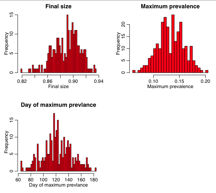
The script also outputs the average value, and 95% CI for each of these model outputs.  The 95% CI is determined from the lower limit that excludes the lowest 2.5% of the distribution, and the upper limit that excludes the upper 2.5% of the distribution.  The R function quantile() helps calculate this.

The R script also uses the Shapiro-Wilk test to see if the distributions of the model outputs are consistent with being Normally distributed.  They certainly don’t have to be, but it is interesting to know if they are.

What we would also like to know is how each of these quantities depends individually on the variance in the various parameters.  Thus the script plots the final size vs each of the parameter hypotheses:

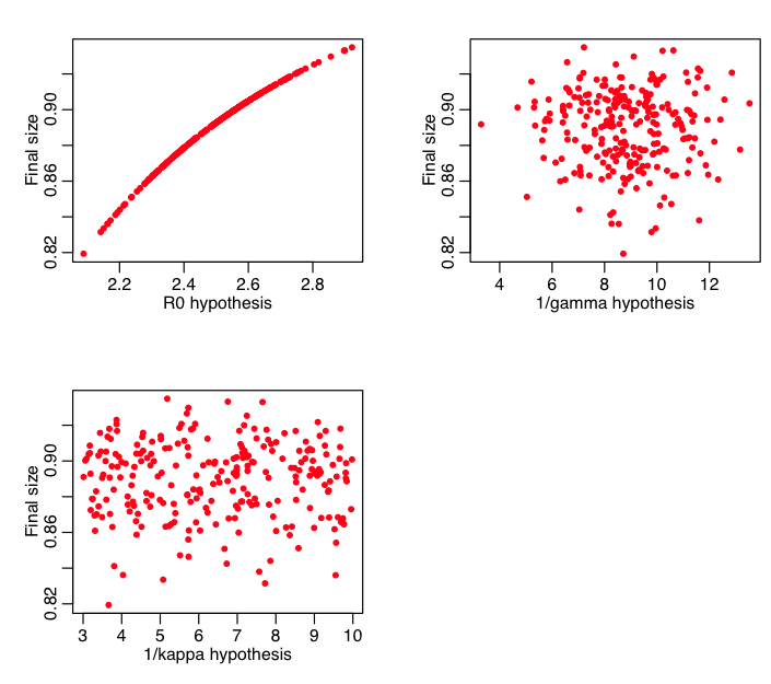
Question: does the final size depend on R0? kappa? gamma?  If so, why? If not, why not?

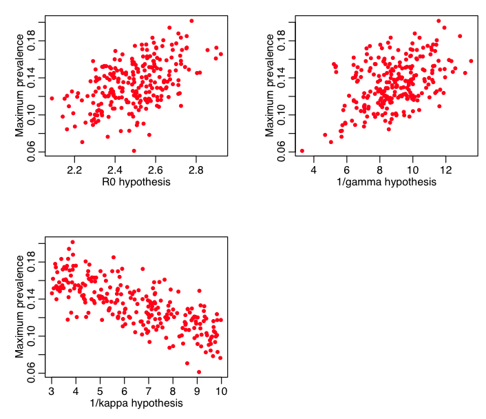
The script also plots the maximum prevalence vs these parameters:

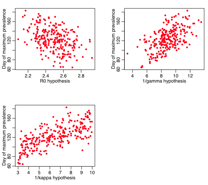
And the day of the maximum prevalence:

You could also use Latin Hypercube Sampling, but shouldn’t

Back in the old-timey days, when computers were a lot slower, it was computationally infeasible to do, say 1000 iterations, of the above procedure.  Instead, what they’d resort to is breaking up the parameter values into discrete values within their range (and, generally, assume Uniform probabilities for each value, but not necessarily).  Then, they’d do an outer loop over the few (N_R0) discrete values of R0, a nested loop over the few discrete values of gamma, and another nested loop over the few discrete values of kappa (thus each of the N_R0*N_gamma*N_kappa combinations of values gets examined only once). 

This is known as Latin Hypercube Sampling.

The problem with this method is that you don’t get a full sense of how the model output varies smoothly with the parameter.  And setting up those loops is clunky.

But if you have very little computing power at your fingertips, LHS is the go-to method.  But even low-end laptops and desktops have more than enough computing power to avoid using LHS these days.

I’ve noticed that even in recent literature authors still claim to use “Latin Hypercube Sampling”, when what they really mean is the non-discrete Monte Carlo sampling procedure that I described above.  For some reason the misnomer gets propagated through modern literature.

When using the non-discrete method I described above, you would describe it in a paper as “To assess the uncertainties on the model outputs, we performed YYY iterations of Monte Carlo sampling of the parameter values from their probability distributions, calculating the model output for each combination of parameter hypotheses.  The resulting distributions of the model outputs are shown in Figure ZZZ” (or just state the average and 95% CI on the model outputs).