
In this module, students will become familiar with population standardized regression methods when working with data that is expressed as per-capita rates
Data that are expressed as per-capita rates are frequently encountered in the life and social sciences. For example the per-capita rate of incidence of a certain disease, or per-capita crime rates. In both examples, “per-capita” means “per person”. And because the per-capita rate is expressed as “per person”, sometimes it might be easy to get confused and think that perhaps Binomial linear regression methods might be most appropriate because the data appear at first blush to be expressed as a fraction of the population.
But you’d be wrong… Binomial linear regression methods are only appropriate for fractions that are strictly constrained to be between 0 and 1. When we are talking about crime rates, for example, it’s entirely possible if crime were rampant that someone might be robbed several times a year. The per-capita annual rate could thus be above 1!
When talking about per-capita rates, the data consist of a counted number per some unit time, thus regression methods like Poisson or Negative Binomial methods would be appropriate. But we have to account for the population size, M, because obviously if the population doubles, the number of cases of crime we would count per unit time would also double (if the per-capita rate stayed the same).
To take this into account in a regression analysis, we use what is called “population-standardized” regression. Recall that Poisson regression methods use a log link for the expected number of events, lambda. In population-standardized linear regression with one explanatory variable (for example) we thus have
![]()
Notice that if we bring the log(M) over the LHS, we get log(lambda/M)… the per-capita rate!
Also notice that the log(M) term does not (nor should it) have a coefficient multiplying it in the fit. Thus, if your observed number of crimes are in the y vector, what you do NOT want to do is the following (recall that the glm function with family=poisson in R uses a log-link by default):
b = glm(y~log(M)+x,family="poisson")
This is because R will attempt to find some kind of best-fit coefficient for the log(M) term, when what we actually need to do is force its coefficient to be 1 to be able to interpret our output as a per-capita rate.
The way to do this in R is to use the offset() function:
b = glm(y~offset(log(M)) + x, family="poisson")
Now, in the fit the log(M) term is forced to have coefficient equal to one.
Here is a 2000 paper by W. Osgoode on the subject of population standardized Poisson regression.
Example
Let’s look at the annual per-capita rates of public mass shootings before, during, and after the Federal Assault Weapons Ban, which was enacted from September 14, 1994 to September 13, 2004. In the file mass_killings_data_1982_to_2017.csv, there is the annual number of public mass shootings from 1982 to 2017, as obtained from the Mother Jones mass shootings data base, and supplemented with a few public mass shootings they missed, as listed in the USA Today mass killings data base. Also in the file is the US population that year (in milliions), as obtained from the US Census Bureau. There is also a logical variable, lperiod, indicating wether the year was before (lperiod=0), during (lperiod=1), or after (lperiod=2) the ban assault (note that lperiod=1 when the weapons ban was in place for most of that particular year). Also included in the file is the number of people killed in mass shootings each year (the last two variables aren’t used in the following example).
The following code reads in this data, and does a population standardized fit, then plots the data and fit results:
adat=read.table("mass_killings_data_1982_to_2017.csv",sep=",",as.is=T,header=T)

b = glm(number_shootings~offset(log(pop)),family="poisson",data=adat)
plot(adat$year,adat$number_shootings,cex=2,xlab="Date",ylab="Number mass shootings")
lines(adat$year,b$fit,col=2,lwd=5)
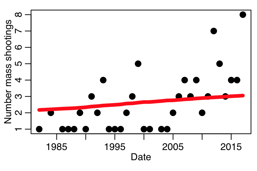
You can see that the fit estimates properly take into account that the US population went up from 1982 to 2017, and thus, even if the per-capita rate were the same over that entire period, we would expect a higher annual number of events in 2017 compared to 1982.
The summary of the fit from summary(b) yields
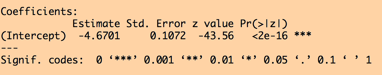
To interpret this output, we note that the glm family=”poisson” fit uses a log link. hus we must take the exponential of the intercept term to get the average expected per-capita annual rate. This is exp(-4.6701)=0.0094 per million people, per year.
We can compare this to what we get if we just take the average of the number of killings per million people per year: mean(adat$number_shootings/adat$pop)=0.0091. The two numbers are almost identical… and they should be!
In the literature, you may see people doing fits to (y/pop) using least squares regression, but that is the wrong method to use because the data will not satisfy the Normality assumption of the least squares method, because the y are Poisson distributed, and simply dividing by A does not magically transform things to make (y/A) Normally distributed.
Other potential types of standardized regression
If one assumes that the population density of some animal (or people) is the same over some study areas, but might depend on time (for example), if the researchers count the individuals, y, in places with areas, A, at distinct points in time, t, they can estimate the change in population density using area standardized regression, using a function call like:
b = glm(y~offset(log(A)) + t, family="poisson")
Note that Poisson regression is the appropriate fitting method to use, because these are count data (and may in fact involve low counts).
Another type of standardized fit might be if a researcher had counts of some organism in different samples of fluid with volumes, V, and wished to see how this might depend on some other explanatory variable.