
Compartmental models of infectious disease transmission inherently assume that the time spent (“sojourn time”) in the infectious state is Exponentially distributed. As we will discuss in this module, this is a highly unrealistic assumption. We will show that the “linear chain rule” can be used to incorporate more realistic probability distributions for state sojourn times into compartmental mathematical models.
A simple example of a compartmental model of infectious disease spread is the Susceptible, Infectious, Recovered model. In several past modules we have discussed this model in detail, but briefly, individuals in the susceptibly compartment can be infected on contact with infectious people in the population (whereupon they flow to the “infectious” compartment). Infectious people recover with some rate, gamma, and flow into the “recovered and immune” compartment.
The compartmental diagram for the model looks like this:
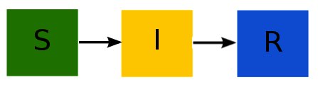
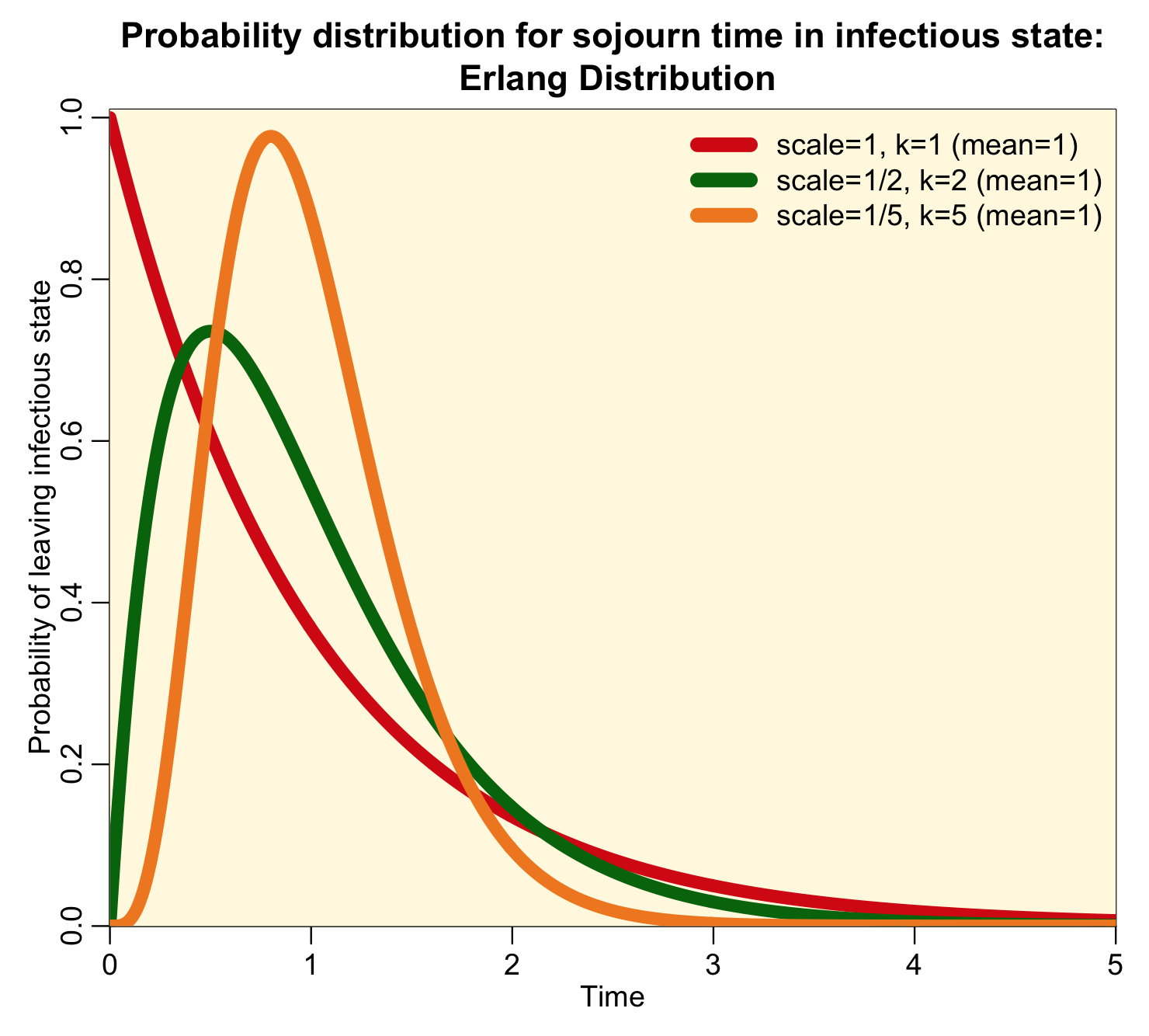
and the system of ordinary differential equations describing these dynamics is:
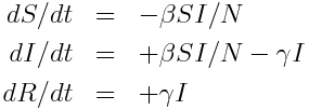
Inherent in these model equations is the assumption that the sojourn time in the infectious compartment is Exponentially distributed, with rate gamma. You can see this if you look near the beginning of the outbreak where I is approximately equal to zero, in which case the equation for dI/dt is dI/dt=-gamma*I. The solution to this equation when I goes to zero as t goes to infinity is I(t) = I_0 exp(-gamma*t).
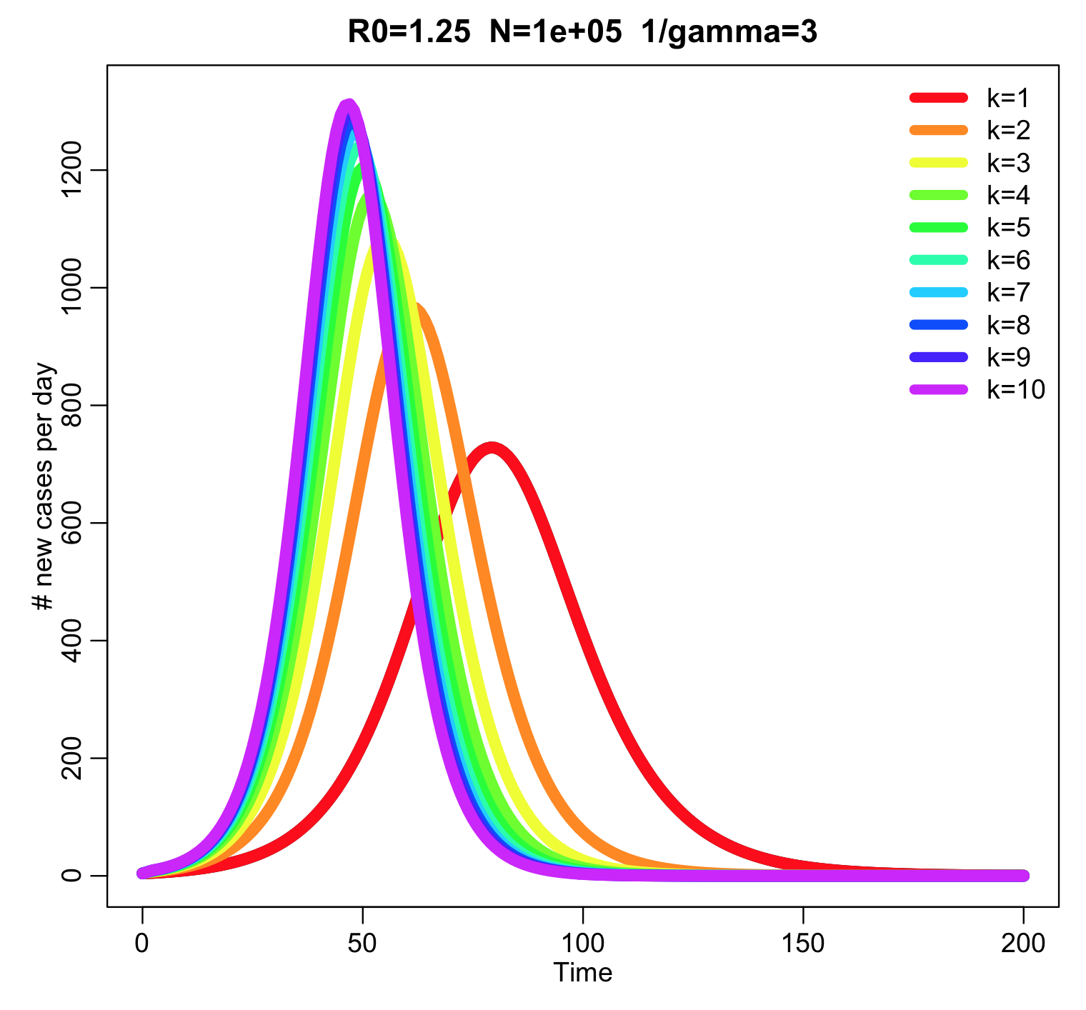
The probability distribution for the sojourn time in the infectious state for this model thus looks like this:
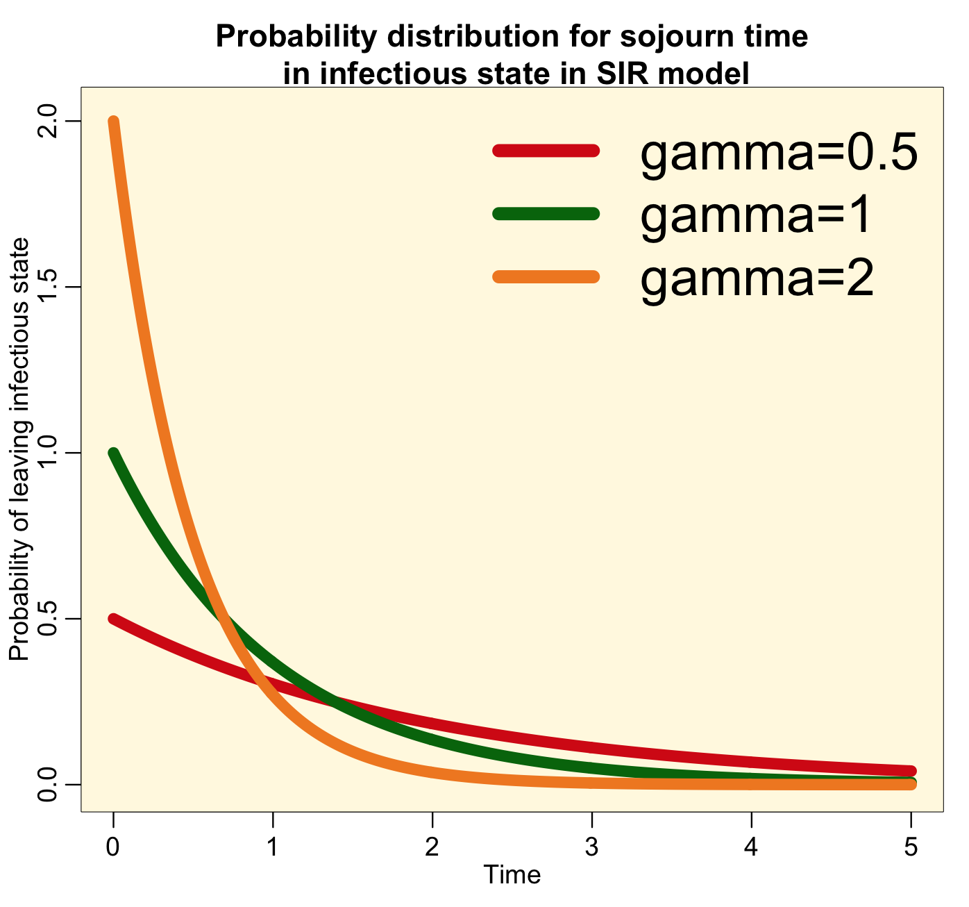
Notice that the most probable time for leaving the infectious state is time t=0. This implies that the most probable time that you will recover from a disease like influenza or measles is immediately after being infected…. this is clearly high unrealistic! For all diseases, realistically, the probability distribution for the sojourn time in the infectious state looks more like a bump, like this:
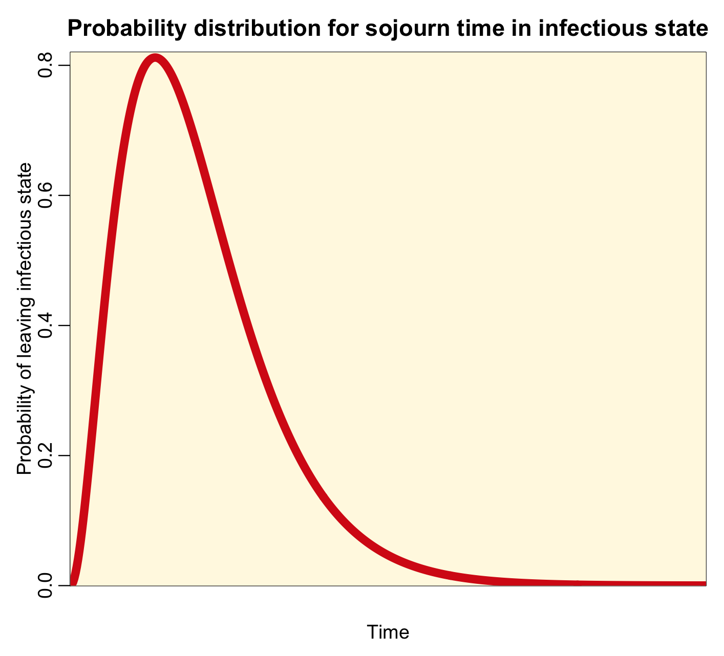
With this distribution, at time t=0, the probability of leaving the infectious state is zero (as it is in reality). A few people recover early on after being infected, but most of those infected recover near the middle of the bump. A few take much longer to recover, and are in the tails of the distribution.
So, how can we incorporate realistic sojourn times like this in compartmental models? And why would we even want to? (hint: think about control strategies, like treatment or isolation, that might be aimed at people at various times after they are first infected… there is often a delay between time of infection and the application of an intervention strategies).
Gamma distributed sojourn times
It turns out the Gamma distribution offers an easy way to incorporate realistic sojourn times in a model. The Gamma distribution has two parameters, a shape parameter, k, and a scale parameter theta. The mean of the distribution is mu=k*theta. The probability density function for the Gamma distribution is:
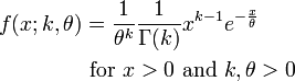
When k is an integer, the distribution is called the Erlang distribution, and for the special case when k=1, the distribution is the Exponential probability distribution. It turns out that an Erlang distributed random number with scale parameter theta is the sum of k Exponentially distributed random numbers with rate theta. Here is an example of how the parameter k affects the shape of the Erlang distribution when scale parameter theta=1/k (and thus the mean of the distribution is one):
Notice that the higher the value of k, the more narrow and peaked the distribution is.
Linear chain trick
Because an Erlang distributed random number with scale theta and shape k is the sum of k Exponentially distributed random numbers with rate theta, there is a method called the “linear chain trick” that adds k disease stages to a compartmental model, each of which flows into the next with rate k*theta (except for the last which flows to the recovered class), where 1/theta is the average infectious period for the disease.
For the SIR model, if we assume the rate is gamma, we get
The R script sir_erlang_sojourn.R shows an example of how to code up a linear-chain model in R. It requires that the sfsmisc and deSolve libaries have been installed on your computer. If they have not, type in your R console
install.packages("sfsmisc","deSolve")
and choose an R repository mirror site close to your location for the download. Then type in your R console
source("sir_erlang_sojourn.R")
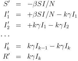
This produces the following plot:
The higher the value of k, the narrower the peak of the outbreak. The script also prints out the final size for the various values of k: the final size of the outbreak is independent of k.
In the absence of births and deaths (vital dynamics) in the model, the reproduction number for this model is exactly the same as a model that that just assumes k=1. That is to say, R0=beta/gamma.
This paper discusses the relationship between R0, k, gamma, and the rate of exponential rise at the beginning of an outbreak for SIR and SEIR models.