[This module compares the results of fitting a model to data when Least Squares,  Poisson and Negative Binomial likelihood statistics are optimized]

Introduction

In a previous module, we explored an example of Least squares fitting the parameters of a mathematical SIR contagion model to data from a real influenza epidemic using the graphical Monte Carlo parameter sampling method.  The R script fit_iteration.R performs the Monte Carlo iterations, randomly sampling values of the reproduction number, R0, and the time of introduction of the virus to the population, t0, from uniform random distributions, calculates the Least Squares statistic, and plots the result to show which value of R0 and t0 minimizes the Least Squares statistic.  The script did not assess the uncertainties on the parameter estimates.

In this past module, we described the use of the other fitting statistics with the graphical Monte Carlo parameter optimisation method, including Poisson and Negative Binomial likelihood statistics, which are appropriate for count data.  The Negative Binomial probability distribution includes an extra parameter that accounts for more over-dispersion in the count data than would be expected from Poisson distributed data.  We discussed in that module the fact that Least Squares statistics are usually not the best choice for use with count data, particularly for count data with widely varying number of counts per bin, and/or just a few counts per bin.

In this past module, we described how you can use the graphical Monte Carlo parameter optimisation method to determine the parameter estimate one-standard deviation uncertainty and 95% confidence interval.  The one standard deviation uncertainty is obtained by looking at the range in sampled parameter values that result in a negative log likelihood statistic within 1/2 of the minimum value of the negative log likelihood (the “fmin+1/2 method”).  The 95% confidence interval is obtained from the range in sampled parameter values that result in a negative log likelihood statistic within 0.5*1.96^2 of the minimum value of the negative log likelihood.

In that past module, we also discussed the fact that the fmin+1/2 method only works when using negative log likelihood goodness-of-fit statistics.  The module described how the Least Squares (LS) statistic is actually equivalent to the Normal negative log likelihood statistic, by using the simple transformation:

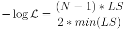 eqn 1

where N is the number of data points being fit to.

In this module, we will compare fitting to the influenza epidemic incidence data recorded during the 2007-2008 season in the Midwest.  We will show examples of using the Least Squares Normal negative log likelihood statistic, Poisson negative log likelihood, and Negative Binomial negative log likelihood.  Because the incidence data are count data, and are almost certainly over-dispersed, the Negative Binomial neg log likelihood statistic is the most appropriate goodness-of-fit statistic.  However, it is instructive to do the fit using Least Squares and Poisson negative log likelihood statistic to compare the best-fit values and confidence intervals on those estimates.

Fitting using the Least Squares Normal negative log-likelihood statistic

The R script fit_iteration_lsq_fmin_plus_half.R fits to the Midwest influenza data contained in the file midwest_influenza_2007_to_2008.dat.  The script does 10,000 iterations randomly sampling values of R0 and the time-of-introduction of the virus to the population, t0, calculating the Least Squares statistic comparing the model and data at each iteration.  After the 10,000 iterations are over, the script calculates the Least Squares Normal negative log likelihood statistic using equation 1 above.

The script then produces the following plots.  The horizontal dotted red lines indicate the (fmin+1/2) and (fmin+0.5*1.96^2) values of the negative log likelihood.  The range of sampled parameters under these lines represent the one standard deviation uncertainty and 95% CI respectively:

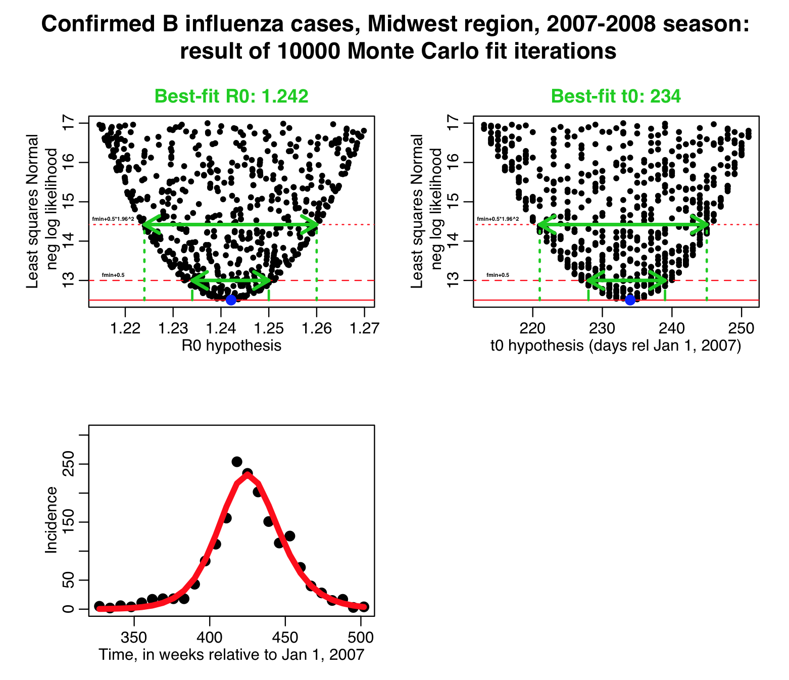
The solid horizontal red line represents the minimum value of the negative log likelihood (“fmin”), and the dashed horizontal red line represents fmin+1/2.  The range of parameter hypotheses under that line is the one standard deviation confidence interval.  The dotted horizontal red line represents fmin+0.5*1.96^2… the range of parameter hypotheses under than line is the 1.96 std deviation confidence interval (aka: the 95% confidence interval).

Based on range of the parameter hypotheses under these lines, the script also outputs the results:

Note: this script does 10,000 iterations of the graphical Monte Carlo method, but in practice the plots of the negative log likelihood versus parameter hypotheses should be more densely populated than what they are here to ensure precise estimation of the best-fit and the confidence intervals on that estimate.

Fitting with a Poisson negative log likelihood fit

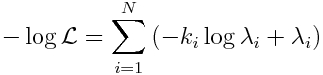
The influenza incidence data are count data and have a large range in the number of counts per bin, from just a few per bin to hundreds in this data sample.  Least Squares is thus not a good choice of a goodness-of-fit statistic for these data.  A goodness-fo-fit statistic specifically for count data would be more appropriate.  The Poisson distribution describes stochasticity in count data, and has one parameter lambda.

The R script fit_iteration_poisson_fmin_plus_half.R does 10,000 iterations randomly sampling values of R0 and t0 at each iteration and calculating the Poisson negative log likelihood statistic:

The script produces the following plot:

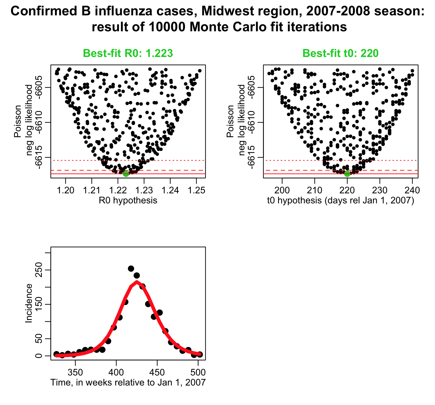
and prints out the following results:

Notice that the one standard deviation uncertainties (and 95% CI) are significantly narrower than those calculated using the Least Squares Normal negative log likelihood fit.  This is because the data are over-dispersed, and the Poisson negative log-likelihood will always underestimate the uncertainties on the parameter estimates for over-dispersed data.  Whatever other drawbacks the Least Squares method has for use with count data, at least it takes into account over-dispersion.

Fitting with a Negative Binomial negative log likelihood fit

As mentioned in this past module, if your research question involves count data, pretty much always such data are over-dispersed, meaning that the stochastic variation in the data is much larger than would be expected from the Poisson distribution.

The R script fit_iteration_negbinom_fmin_plus_half.R does 50,000 iterations (it will take a while to run) sampling values of R0, t0, and the over-dispersion parameter alpha at each iteration. The reason more iterations are needed is because three parameters are now being fit for rather than two…. the more parameters you fit for, the more iterations you need to do in the graphical Monte Carlo method to reliably estimate the best-fit values and their uncertainties.

The R script uses two functions I provide my_dnbinom(), and my_lnbinom().  The my_lnbinom() function takes as its arguments the data, the predicted model, and an estimate of the over-dispersion parameter, and calculates the Negative Binomial negative log-likelihood statistic.  When doing your own Negative Binomial likelihood fits, use these two functions.  I have put them in the file negative_binomial_likelihood_calculation_functions.R for you.

The fit_iteration_negbinom_fmin_plus_half.R  script produces the plot:

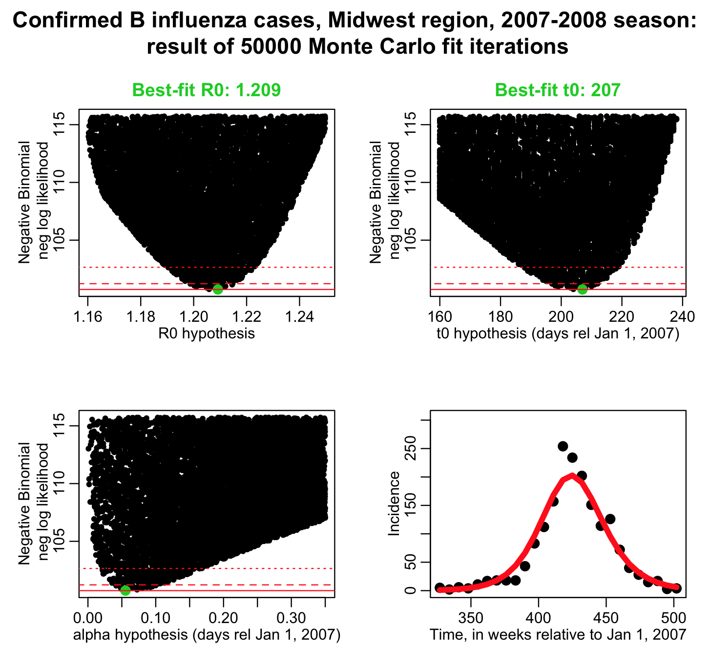
and produces the output:

Compare this to the estimates from the Least Squares Normal negative log likelihood fit:

The uncertainties from the Negative Binomial likelihood fit are approximately comparable in size to those obtained from the Least Squares fit, but the best-fit estimates are quite different.  Inappropriate use of Least Squares can lead to biased parameter estimates.

Note that we usually don’t bother reporting the estimates of the over-dispersion parameter, alpha.  It is a nuisance parameter we have to fit for, but beyond checking that it isn’t statistically consistent with zero, it isn’t interesting.  Note that “statistically consistent with zero” means that the value of zero lies within the 95% confidence interval; if this is the case, then you are justified in using a Poisson likelihood fit.

Summary

Many of the problems we encounter in our research questions involve integer count data.  In this module, we discussed that Least Squares probably isn’t the best choice for such data due to heteroskedasticity (however, you will see in the literature examples where people apply LS fits to count data anyway!).  Inappropriate uses of the LS statistic should be caught in review, but often aren’t.

If the count data involve low-counts, a better choice is the Poisson negative log-likelihood (and at times you see such fits in the literature too), but count data are usually over-dispersed, in which case the best choice always is the Negative Binomial negative log-likelihood.  In fact, in general, the Negative Binomial statistic is always applicable to independent count data, whereas the other three statistics we discuss here each have limitations in their applicability.

The only draw back of using the Negative Binomial likelihood is that it requires fitting for an extra parameter, the over-dispersion parameter alpha, and the mathematical expression of the statistic looks complicated and involved, and can potentially scare the bejeezuz out of reviewers of your papers.  Don’t let that stop you from using it though.  Simply cite well-written papers like the following as precedent for using NB likelihood for count data in the life and social sciences, and perhaps consider not writing the explicit formula for the NB likelihood in your paper… just mention that you used it: Maximum Likelihood Estimation of the Negative Binomial Dispersion Parameter for Highly Overdispersed Data, with Applications to Infectious Diseases.

If you want to get your work published in a timely fashion, strive to use methods that are rigorous, but as simple as possible.  If you have to use a more complicated method, describe it in your paper in plain and simple terms.  In my long experience, this can avoid many problems with things getting hung up unnecessarily long times in review.