[In this module, students will become familiar with estimating parameter confidence intervals when using the Monte Carlo method to estimate the best-fit parameters of a mathematical model to data.]

• Introduction
• Local curvature of likelihood GoF statistic close to minimum, and relationship to parameter uncertainties
• Estimating parameter uncertainties with the Hessian matrix
• A more simple method for estimating parameter uncertainties: the fmin plus a half method (aka graphical Monte Carlo method)
• Using the graphical Monte Carlo method with Least Squares
• Constructing 95% Confidence Intervals
• Example to show that graphical Monte Carlo method actually works

Introduction

As mentioned in previous modules, parameter estimation involves not just estimating the central value, but also your uncertainty on the estimate.  This is because data have stochasticity (randomness), and this randomness translates into uncertainty on our model parameter estimates.  The more stochasticity in the data, the larger the uncertainty on the parameter estimates.  Unless specifically told otherwise, parameter uncertainties are assumed to be Normally distributed.

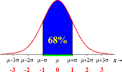
The one standard deviation confidence interval on average contains the true parameter around 68% of the time.   This comes from the properties of the Normal distribution: 68% of the area under the distribution lies between +/- 1 std deviation from the mean:

A wide confidence interval indicates that there is a large amount of uncertainty on the parameter.

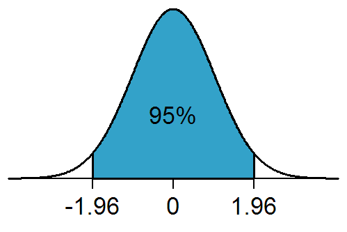
While quoting one standard deviations on estimates is often seen in the literature, so is quoting the 95% confidence interval. The 95% confidence interval on average contains the true parameter estimate 95% of the time.  

The 95% confidence interval is equivalent to the 1.96 standard deviation confidence interval (because 95% of the area under the Normal distribution lies between -1.96*sigma to +1.96*sigma, where sigma is the one standard deviation width of the Normal distribution)…. sometimes people round up and just quote the 2 std deviation confidence interval as the 95% CI.

In this module we’ll assume that either a Monte Carlo parameter random sampling, Latin Hypercube, or Markov Chain Monte Carlo method was used to sample parameter hypotheses, calculate the model, and then calculate a goodness-of-fit statistic comparing the model to the data.  With those methods, we’ll see below that there is a simple graphical method for determining the uncertainties on parameter estimates.

Again, as we’ve repeatedly discussed in previous modules, before you proceed with any parameter estimation (and confidence interval estimation) you have to be careful that your goodness-of-fit statistic is appropriate to your data.  For instance, the Pearson chi^2 weighted least squares goodness-of-fit statistic is appropriate for count data.  The Least Squares statistic can be used with many types of data, including count data (as long as the number of counts don’t vary widely, and the minimum number of counts is at least 10).  The Poisson and Negative Binomial negative log likelihood statistics are appropriate for count data. The Binomial negative log likelihood statistic is appropriate for prevalence data.

Local curvature about the minimum of the goodness of fit statistic, and how this relates to parameter uncertainties

As described in previous modules, with our Monte Carlo parameter random sampling procedure, we search for the parameters that minimize our goodness-of-fit statistic (let’s call it “f”… “f” could be, for example, the Least Squares, Pearson chi^2, or Poisson negative log likelihood statistics).  To locate the minimum, we make plots, like the one below, of the goodness of fit statistic vs the parameter hypothesis.

It should be obvious to the reader that the more sharply curved the plot is close to the minimum, the smaller the uncertainty in that model parameter estimate (because a small change in the model parameter results in a big change in “f”). Here is an example:

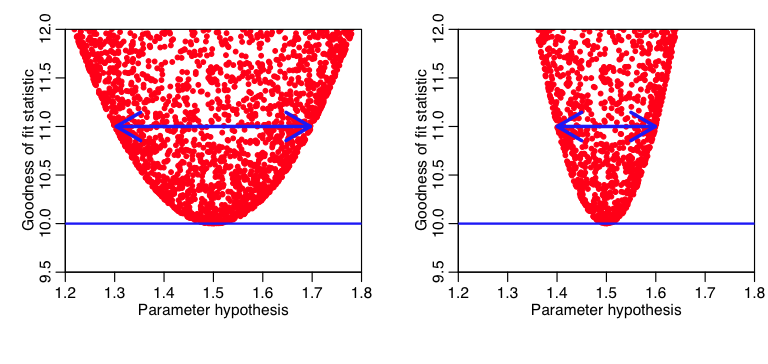
Note that if we go up a difference of one (for instance) from the minimum value of the GoF statistic, we see that the plot on the left is much more gently curved than the one on the right (ie; the range of the parameter hypotheses at that point is much wider in the plot on the left compared to the one on the right).  The parameter estimate on the right thus has a smaller uncertainty than the one on the left.

Estimation of parameter uncertainties using the Hessian matrix

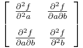
Now, hearken back to your undergraduate multivariate calculus days, and recall that the Hessian matrix is a square matrix of the second order partial derivatives of a multivariate function, f, and describes the local curvature of the function:

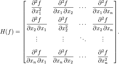
The Hessian is especially useful in quantifying how “sharp” an extremum in the function is. The more sharply a function curves locally for one or more of the variables, the larger the corresponding diagonal elements of the Hessian matrix.

It should not come as a surprise to you that the Hessian matrix is intimately related to the uncertainty on the parameters….  In fact, if the goodness of fit statistic is a likelihood (like, for instance the Poisson or Negative Binomial likelihoods), the covariance matrix for the parameter uncertainties is the inverse of the Hessian (see, for instance, section 5 of this document).

Unfortunately, estimating the Hessian can be a pain, especially considering that because models we normally deal with in this field have no analytic expression for the model estimate, let alone its partial derivatives wrt the model parameters (and recall that the likelihood is calculated from the data and model, and thus it too is a function of the model parameters with no analytic expression).  There are numerical methods that can be used, and it certainly is possible to numerically estimate the Hessian, but it isn’t quite a trivial process.  Despite this, some people prefer to calculate the uncertainty on the parameter estimates using the Hessian, and that’s OK.  I myself prefer a simpler graphical method that is used in particle physics, but I haven’t seen widely applied (yet) in other fields…

A simple method for estimating parameter uncertainties: likelihood GoF statistic and the f_min plus a half method

It turns out that when we are using the Monte Carlo parameter random sampling procedure and have a likelihood goodness-of-fit statistic, there is a very simple way to estimate the parameter uncertainties that doesn’t involve calculating the Hessian; as long as our data samples are large (ie; you will need to be fitting to more than just a few data points), then our likelihood statistic approaches a multivariate Normal distribution in the parameter hypotheses. There is more than an entire course worth of statistical theory behind that statement, and going into much of the background is beyond the scope of this course, but I’ll describe it’s derivation in brief in just a moment.

Here is what that statement implies if we are fitting for just one parameter, theta:

where theta_0 is the best-fit parameter, and sigma is its one standard deviation uncertainty.  Recall that we normally deal with negative log likelihoods.  Thus this reduces to

       Eqn 1

Notice that this is a parabola.  This is why, when we plot -log(L) vs parameter hypotheses, theta when we are only fitting for one parameter, we get a parabola.  If we are fitting for more than one parameter, Eqn 1 turns into a multi-dimensional paraboloid, and that’s why we see parabolic “envelopes” on our plots of -log(L) vs parameter hypotheses.

Simply put, this statement is derived from the second order Taylor expansion of the log likelihood about the best estimate of the parameter, hat(theta) (see section 6.5 of this awesome reference on topics of statistical data analysis):

when the log likelihood is maximized (ie; when theta=hat(theta)), the second term is zero (because it involves the first derivative).  And we recognize the coefficient of the third term as the Hessian, which, from above we know for a one-dimensional problem is 1 over the parameter uncertainty (ie; it is 1/sigma^2).

I think it is so cool that such a simple parabolic expression can be derived for the shape of our negative log likelihood curve close to the minimum… again, to re-iterate, this is the reason that our plots of the negative log likelihood vs the parameter hypotheses have that parabolic envelope!

Now, take a look at Eqn 1 again (recalling that theta_0 is the best-fit value of theta):

It should be clear that if we take theta=theta_0+sigma (or theta=theta_0-sigma) then the negative log likelihood (let’s call it “f”) shifts up by a half from its minimum value.

And here is where the beauty of this lies; if we take our plots of the negative log likelihood vs parameter hypothesis, and draw a line up 0.5 from the minimum value of -log(L), the range of points under that line is our one standard deviation confidence interval. It turns out this works even when we are fitting for multiple parameters.  This provides a really easy graphical way to estimate our confidence intervals!

Here is the recipe:

1. Do your Monte Carlo iterations randomly sampling parameter hypotheses, calculate your model estimates with the parameter hypotheses, and calculate the resulting negative log-likelihood statistic.
2. Make the plots of the negative log likelihood statistic vs your parameter hypotheses.
3. You will estimate the parameter one standard deviation confidence interval by going up 1/2 from the minimum value of the negative log likelihood statistic (hence the fmin plus a half moniker I’ve given this method), and looking at the range of parameter hypotheses that lie below that line.

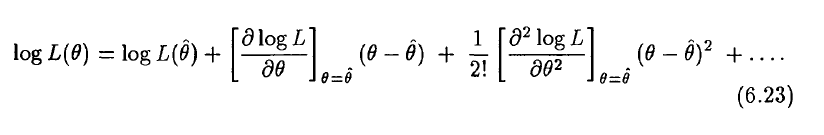
And here is an example of what it looks like in practice.  This R script fit_flu_data_poisson.R fits to the Midwestern B influenza incidence data during the 2007-08 influenza season.  It does 10000 iterations of a Monte Carlo parameter sampling procedure, where it randomly samples the R0 and time-of-introduction for an SIR model, then calculates the Poisson negative log-likelihood statistic comparing the model to the data.  It produces the following plot:

The script also outputs the parameter hypotheses and the corresponding Poisson negative log-likelihood values to the file results_of_poisson_likelihood_fit_to_midwest_flu_data.csv

The R script determine_confidence_intervals.R  reads in this output data and calculates the parameter estimates and the one standard deviation confidence intervals.  You will need to install the scatterplot3d library in order to run it.

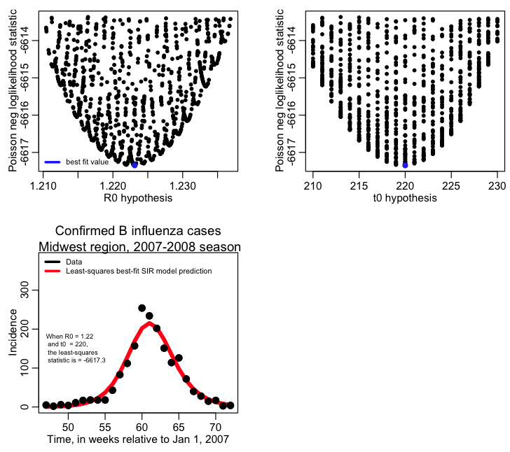
The first plot it produces is a 3D plot of the value of the Poisson negative log likelihood vs the R0 and t0 parameter hypotheses.  Can you see that it forms a 3D parabolic surface?

When you are fitting multiple parameters, the likelihood vs the parameter hypotheses forms a multidimensional parabolic surface.  When you plot the likelihood vs one of the parameter hypotheses, you are projecting all these points onto that plane.

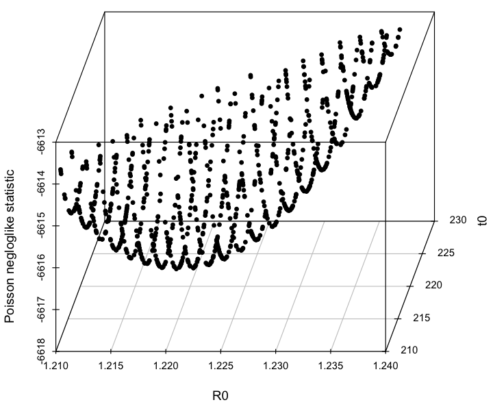
The script also produces the following plot, showing how the confidence intervals are estimated:

(figure 1)

The best fit estimate for R0 is 1.223 with 1 std dev confidence interval [1.218,1.227].

The best fit estimate for t0 is 220, with 1 std dev confidence interval [216,223].

Based on the plot above, we can see that a problem with these confidence intervals is that we really haven’t run enough Monte Carlo iterations to get a good estimate of the parabolic envelope.  In general, if you run too few Monte Carlo iterations, you are likely to underestimate confidence intervals.

Also, the Poisson negative log likelihood is not the most approriate likelihood statistic we could use with this data.  Instead we should account for over-dispersion in the data by doing a Negative Binomial log-likelihood fit.

This method is widely used in Particle Physics, but for some reason I haven’t seen it used anywhere else even though it is such a simple and elegant method for obtaining parameter confidence intervals.  In Glen Cowan’s statistical data analysis book, he refers to it as the graphical Monte Carlo method (“Monte Carlo” refers to the random sampling of the parameter hypotheses).  Even though physicists use the method fairly often, it isn’t talked about in their papers for much the same reason that we don’t normally discuss the standard methods we might use to solve an integral when we are writing a mathematics paper on some topic (for instance)…. it is just considered common knowledge in the field.

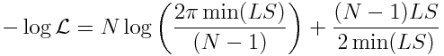
How to make the fmin plus a half method work with Least Squares

If you are using Least Squares as your goodness-of-fit statistic, you are assuming that the data are homoscedastic, and Normally distributed about the true model estimates, with standard deviation sigma.  Always be careful to check that this appears to be the case by plotting the time series of your residuals data minus the best-fit model estimate, and also histogramming the residuals.  The former should not show any obvious temporal patterns in the width of scatter in the points, and the latter should produce a more-or-less Normally distributed histogram.

The standard deviation width of the (Ydata-Ymodel) histogram is the estimate for sigma.  Thus sigma is

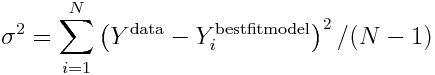 Eqn 2

Now, recall that the Least Squares statistic is

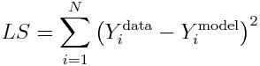
and when Ymodel=Ybest_fit_model, the LS statistic is minimized.

Thus, the minimum value of the Least Squares statistic is

Substituting this into our expression for sigma in Eqn 2 yields

   Eqn 3

So, once you’ve found the best-fit model, you can estimate the stochastic variation in the data from the minimum value of the Least Squares statistic (which is just the sum of the residuals squared, so it makes sense that this is true).

Now, let’s use the fact that the data are Normally distributed, to derive the likelihood for observing our data:

 

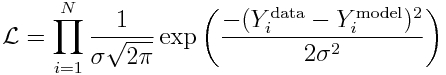
and recall that to reduce computational underflow problems we usually deal with the negative log likelihood, which yields:

 

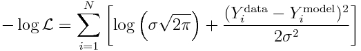
Because sigma is the same for all points, it should be clear that minimizing the Least Squares statistic also minimizes this negative log likelihood!

We know what sigma is from Eqn 3 above.  So we can substitute it in to yield (ignoring the log(2*pi) term):

   Eqn 4

So now we have a likelihood expression, and so we can use our f_min plus a half method to assess the uncertainties on our parameter estimates.  Thus, if you want to estimate the parameter uncertainties using the Least Squares goodness of fit statistic, do the following:

1. Do your many Monte Carlo iterations, randomly sampling the parameters, calculate your model estimates with the parameter hypotheses, and calculate the resulting LS statistic.
2. Once you’ve finished all the many iterations of your Monte Carlo parameter sampling procedure, find the minimum value of your LS statistic.
3. Now, estimate your negative log likelihood statistic using Eqn 3 above (remember, N is the number of data points you are fitting to).
4. Make the plots of this negative log likelihood statistic vs your parameter hypotheses.
5. You will estimate the parameter one standard deviation confidence interval by going up 1/2 from the minimum value of the negative log likelihood statistic, and looking at the range of parameter hypotheses that lie below that line.

 

Obtaining 95% confidence intervals

The Normal distribution has 95% of its area between -1.96*sigma to +1.96*sigma.  Obtaining the 95% confidence interval on a parameter is thus sometimes referred to as the 1.96 standard-deviation confidence interval (and in fact, some people just round it to two standard deviations, and call that the 95% CI).  To obtain an S-standard-deviation confidence interval when using the Monte Carlo parameter parameter sampling method, instead of going up by a half from fmin, you need to go up by 0.5*S^2, and look at the range of parameter hypotheses that lies beneath that line.  So, for the 1.96 standard deviation confidence interval, instead of going up f_min+1/2, we’d look at the range of points going up f_min+0.5*1.96^2=f_min+1.92

An example showing that the graphical Monte Carlo method is indeed equivalent to confidence interval estimation using the Hessian

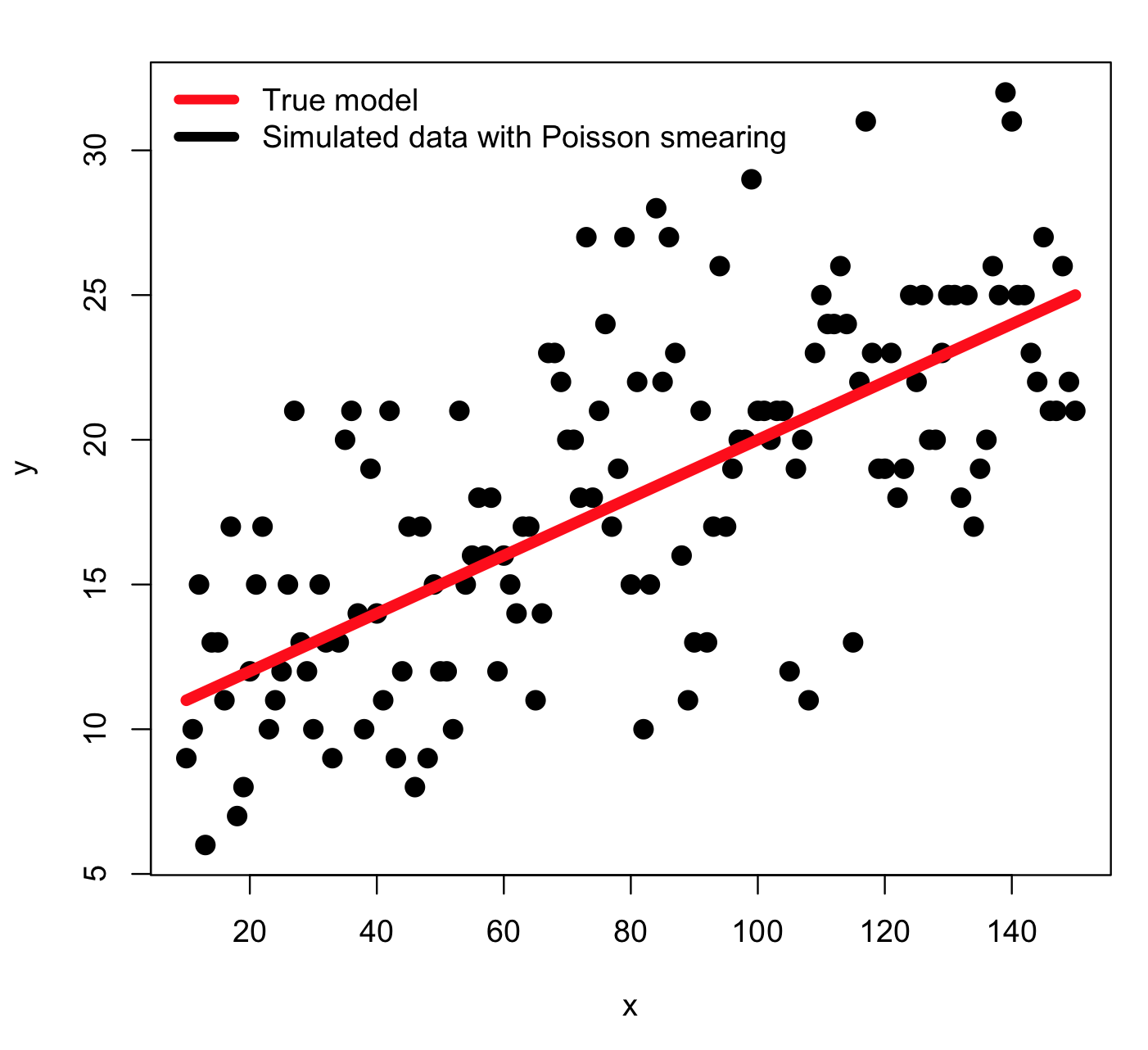
As an example to show that the f_min plus a half method really does work as advertised, let’s consider a simple model for which we can actually calculate an analytic expression for the Hessian.

The model we will consider is y=a*x+b, where a=0.1 and b=10, and x goes from 10 to 150, in integer increments.  I will simulate the stochasticity in the data by smearing with numbers drawn from the Poisson distribution with mean equal to the model prediction (is it clear that an obvious choice of GoF statistic for this simulated data is the Poisson negative log likelihood?).  Thus, an example of the simulated data look like this:

Recall that the Poisson negative log likelihood looks like this

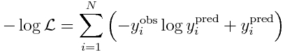
where the y_i^obs are our data observations, and y_i^pred are our model prediction (y_i^pred = a*x_i+b).

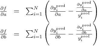
It should be obvious that we can readily calculate the double partial derivatives of -log(L) wrt a and b in order to obtain the Hessian. This first involves calculating the partial derivatives of y_i^pred wrt to a and b, like so:

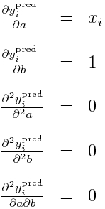
Now, calculate the partials of our negative log-likelihood (let’s call it f, to shorten up the notation):

and then the double partials:

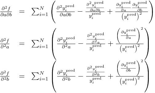
Now, all the double partials of y_i^pred are zero, so this means these double partials simplify to:

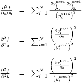
Subbing in our partial derivatives for y_i from above yields:

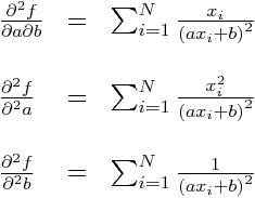
The Hessian matrix for our negative log likelihood is:

In the vicinity of the best-fit a and b, the inverse of the Hessian is the covariance matrix for a and b, and the square root of the diagonals of the inverse are the uncertainties on a and b.

We can randomly generate many different samples of our y^obs, and then use the Monte Carlo parameter sampling method to find the values of a and b that minimize the negative log likelihood.  Then we can calculate the Hessian about this minimum and estimate the one-standard deviation uncertainties on a and b.

 

We can also do this using the fmin plus a half method.  If the fmin plus a half method works, the two estimates for the one-standard-deviation confidence intervals should be very close.

The R script hess.R does exactly this.  It randomly generates 100 different simulated data samples (“simulated experiments”), and uses the Monte Carlo parameter sampling method to estimate a and b for each sample, and also calculates the one-standard-deviation uncertainties based on the Hessian and fmin plus a half method.  It generates the following plot (warning: the script takes awhile to run because it fits to so many samples):

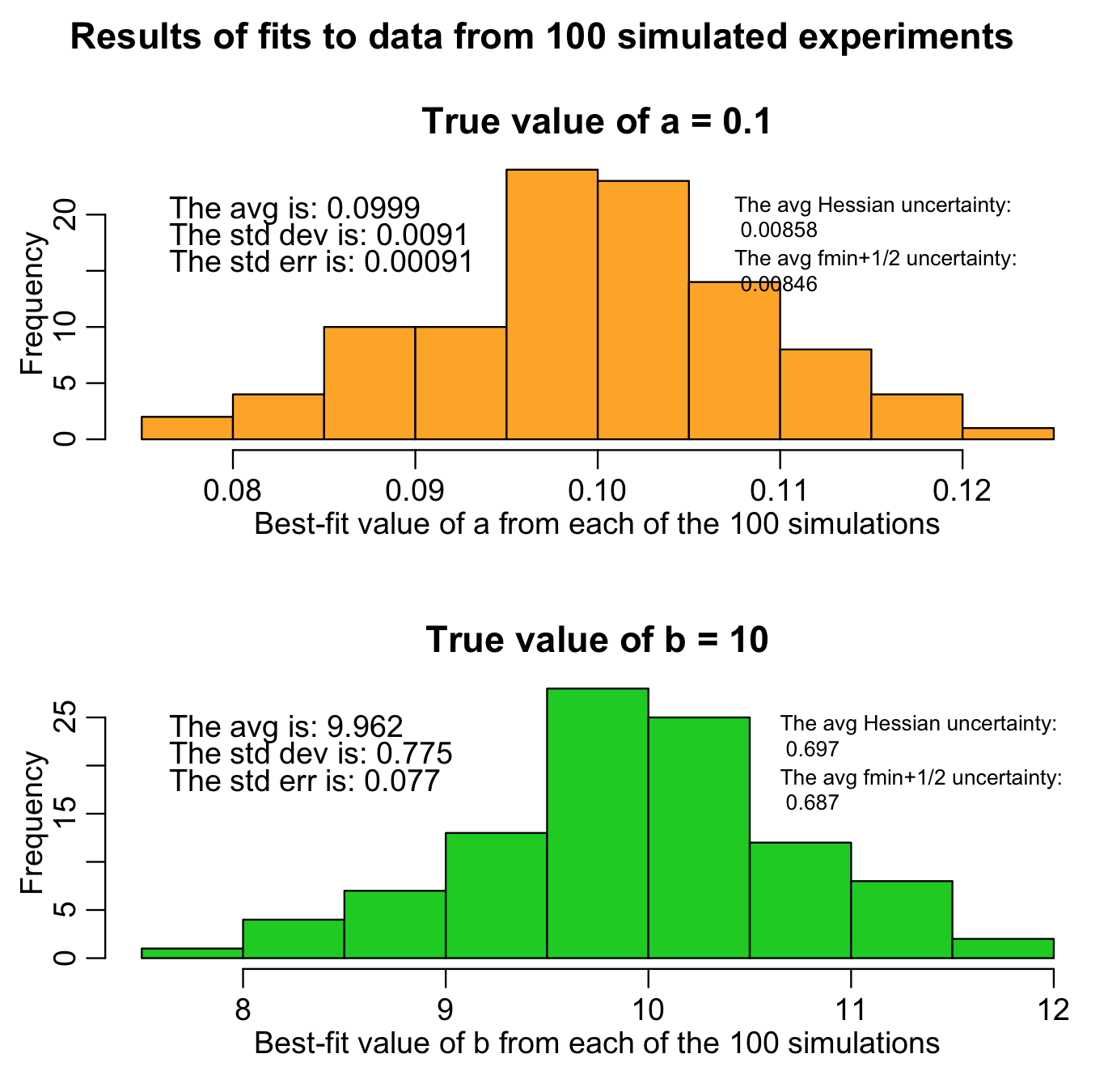
The histograms are the histograms of the best-fit estimates of a and b from each of our 100 different “experiments”.  The average of both should be close to the true values (and, in fact, we can use the Student’s t-test with the observed mean and standard error on the mean to test if the means are statistically consistent with the expected values).  Unbiased estimates are desirable.

Notice that both the Hessian and f_min+1/2 methods give similar estimates of the uncertainty, and those estimates are close to the standard deviation widths of the estimates for a and b.  Ideally, they should be consistent with the standard deviation width of the estimates.  This is what is known as “efficiency” in parameter uncertainty estimation.  If you use a goodness-of-fit statistic that is inappropriate for the stochasticity in the data (for instance, using Pearson chi-squared for over-dispersed count data, when a much better choice would be Negative Binomial likelihood), your estimates of parameter uncertainties won’t be efficient.

The script also returns the following plot: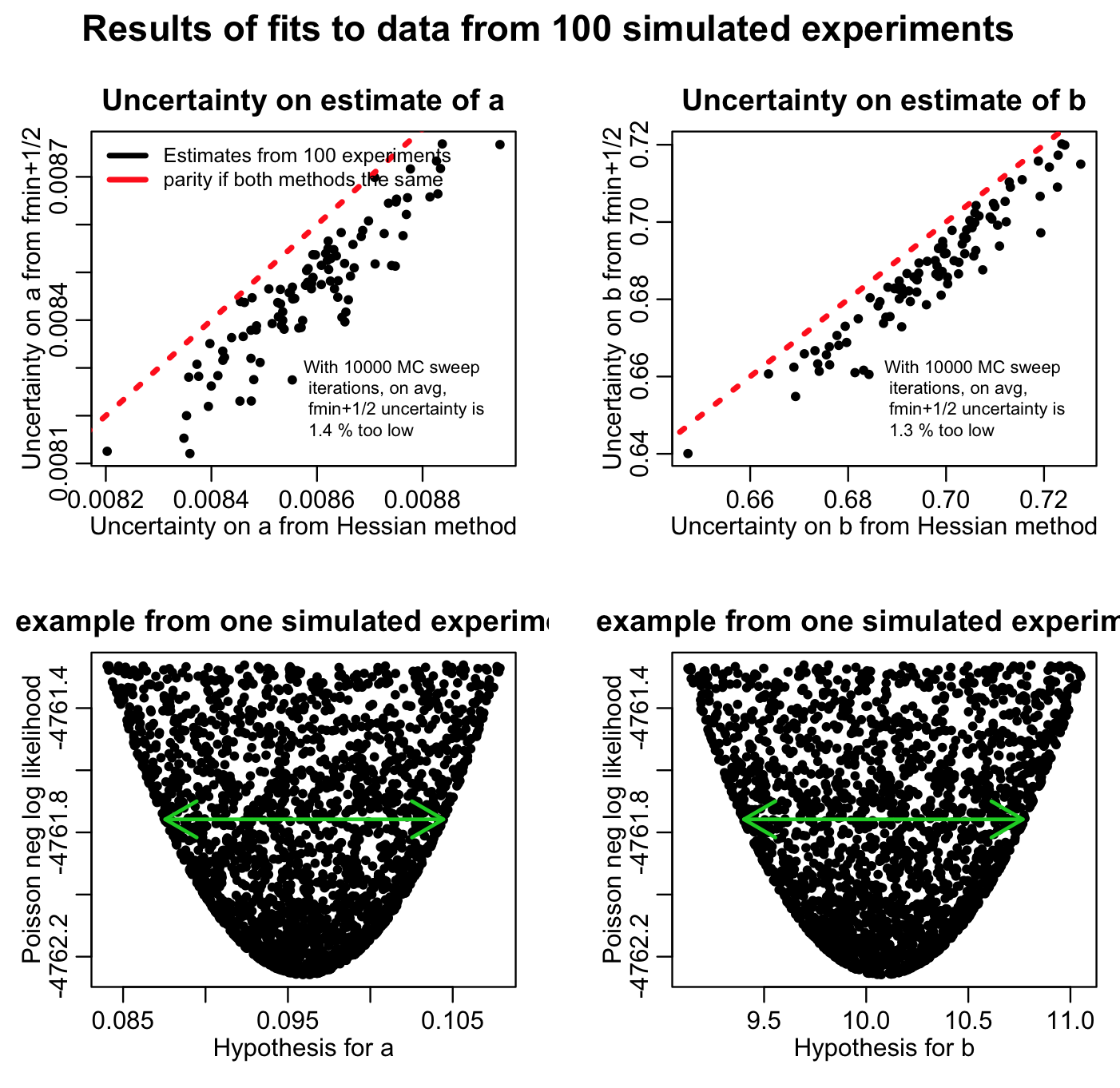

You’ll note that the fmin plus a half method always returns a slightly narrower confidence interval than the estimate from the Hessian matrix (on average there is a relative difference between the two of around than 1%).  This is because if you don’t do enough Monte Carlo parameter samplings, the length of the green arrow denoting the fmin+1/2 method will always undershoot the true width of the parabolic envelope.  This is why you need to do enough Monte Carlo parameter samplings to really populate that plot… ideally, the points should be so dense that the parabolic shape should look black.  The more Monte Carlo samplings you do, the results of the  fmin+1/2 method asymptotically approach the results of using the Hessian matrix.

Is it clear from Figure 1 above that if you do enough Monte Carlo parameter samplings the method will asymptotically approach the estimate from the Hessian matrix?  This is why it is important to do lots of Monte Carlo parameter samplings, which is why it is important to learn how to use high performance computing methods to do this procedure if you are working on a problem that requires estimation of many parameters at once.

Note that our estimates of a and b are not exactly equal to the true values (because of the stochasticity in the data).  Also note that the one-standard deviation of these estimates is very close to the average one-standard-deviation estimate from the fmin plus a half method (and the Hessian method).  This is a further sign that the fmin plus a half method is returning reliable confidence intervals!

Note that if your likelihood function was inappropriate to your data (for instance, using a Poisson likelihood with over-dispersed data), neither the Hessian nor the fmin plus a half methods will return the correct confidence intervals.