[After reading this module, students should understand the Least Squares goodness-of-fit statistic.   Students will be able to read an influenza data set from a comma delimited file into R, and understand the basic steps involved in the graphical Monte Carlo method to fit an SIR model to the data to estimate the R0 of the influenza strain by minimizing the Least Squares statistic.  Students will be aware that parameter estimates have uncertainties associated with them due to stochasticity (randomness) in the data.]

A really good reference for statistical data analysis (including fitting) is Statistical Data Analysis, by G.Cowan.

Contents:

• Introduction
• Least squares goodness-of-fit statistic
• Finding the model parameters that minimize the Least Squares statistic: why we can’t just use linear regression methods for the models we usually use 
• Monte Carlo parameter sweep method
• R code to fit to 2007-2008 confirmed influenza cases in Midwest
• Parameter estimates have uncertainties
• Potential pitfalls of using Least Squares

Introduction

When a new virus starts circulating in the population, one of the first questions that epidemiologists and public health officials want answered is the value of the reproduction number of the spread of the disease in the population (see, for instance, here and here).

The length of the infectious period can roughly be estimated from observational studies of infected people, but the reproduction number can only be estimated by examination of the spread of the disease in the population.  When early data in an epidemic is being used to estimate the reproduction number, I usually refer to this as “real-time” parameter estimation (ie; the epidemic is still ongoing at the time of estimation).

For more common infectious diseases with epidemics that happen on a regular basis, estimating the reproduction number can be done by fitting a disease model to the entire epidemic curve. I often refer to this as “retrospective” parameter estimate, because the epidemic has already run its course (for example, see here)

In this module, I will be discussing retrospective estimation, and leave the topic of real-time estimation during the exponential rise to a later module.  However, one thing that is common to both is that a model is compared to the data, and a “figure-of-merit” goodness-of-fit statistic is calculated that assesses how well the model describes (ie; fits) the data.  In this module I will discuss one such figure-of-merit; the least squares statistic, since it is intuitively the easiest to understand (but, as we’ll see, isn’t applicable to all data, and actually isn’t suitable to the data we fit to here… but it is good enough for expository purposes).

In later modules we’ll discuss the Pearson chi-squared and maximum likelihood figure-of-merit statistics.  In particular, the Poisson maximum likelihood or Negative Binomial likelihood statistics are more appropriate in this case because the data are count data.

No matter what the figure-of-merit statistic you use, you need to ensure that the model you are fitting to your data is actually appropriate to the data! If the model is not appropriate for simulating the underlying dynamics of the system, the answers you get out will be garbage.

Least Squares goodness-of-fit statistic

One of the most commonly used goodness-of-fit statistics is the Least Squares statistic.  It’s the one you learn about when you first learn about linear regression in a Stats 101 course.

This statistic finds the model parameters that minimize the sum of the squared point-by-point distances between the model prediction and the data, as illustrated in this figure: This figure was created by the R script fit_example.R. In order to run it you need to have the deSolve package installed in R for solving the SIR model ODE’s.  You will also need to have the R packages called “chron” and “sfsmisc” installed. If you don’t have them, type in your R command line:

install.packages("chron")
install.packages("sfsmisc")

and pick a mirror site close to your location for installation.   The fit_example.R script also requires that you have already downloaded to your working directory the comma delimited data file I prepared that contains CDC influenza data from the Midwest for the 2007-2008 season, midwest_influenza_2007_to_2008.dat  You also need to download the script sir_func.R, which contains a function that calculates the derivatives in the SIR model equations.

In the fit_example.R script I get the estimated incidence from an SIR model, with population size equal to the population of the Midwest, and assuming that one infected person is introduced into a completely susceptible population at time t0 (is this a good assumption?).  The script assumes that t0 is week 44 of the year, and that the R0 of the epidemic is 1.35.  I assume that the infectious period for flu is 1/gamma=3 days. In this example we assume that there is just one infected person at time t0, and that the population was fully immune.  In reality, those initial conditions are also unknown model parameters that need to be estimated or the assumptions clearly stated.

The script produces the following plot: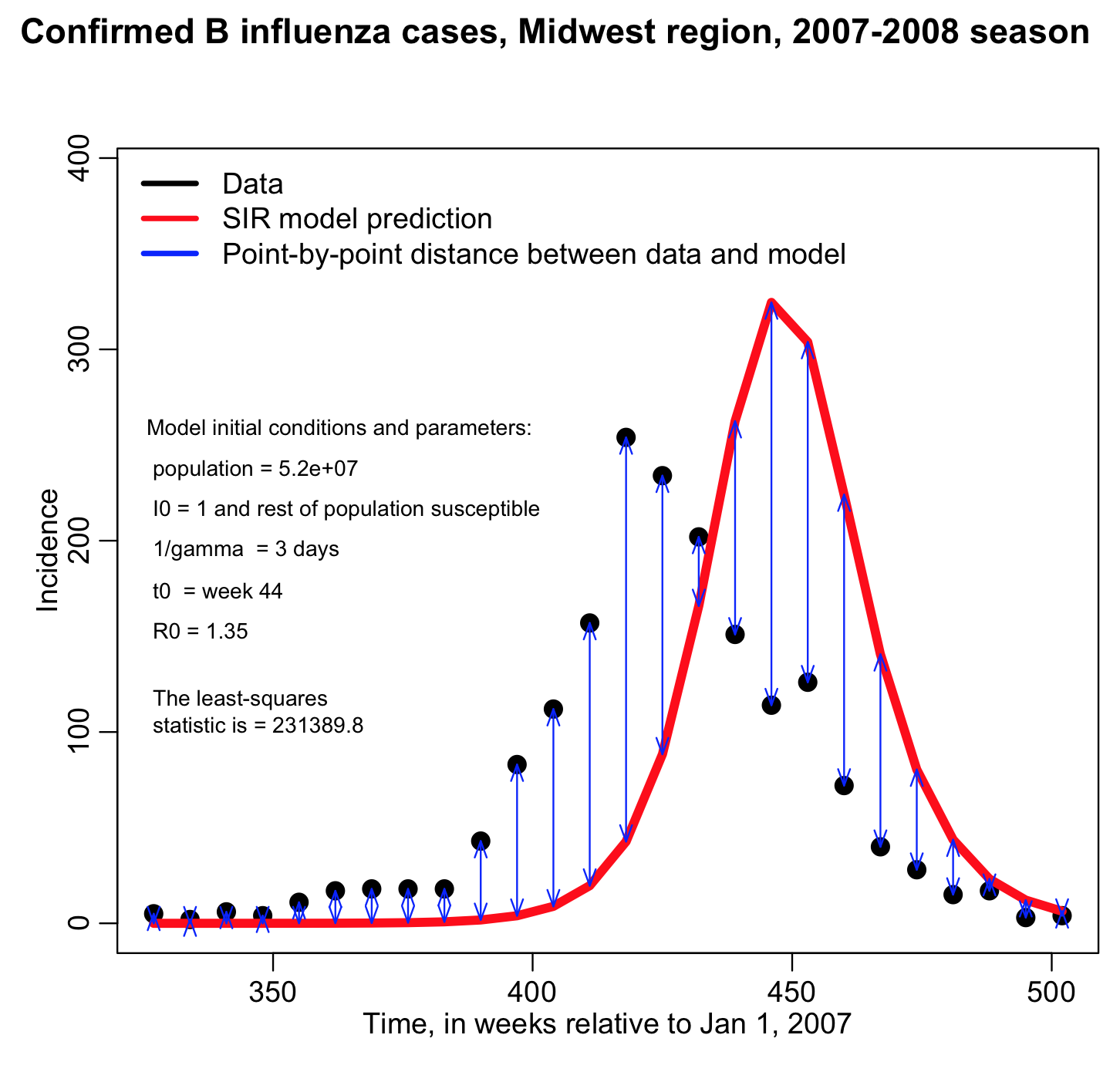

Can you see that a good fit to the data will minimize the sum of the squared distances represented by the blue lines in the plot? The best fit minimizes the least squares figure-of-merit statistic.

If you have n data points Y_i (where i=1,…,n), and model predictions for those data points, model_i (note that these predictions depend on the model parameters!), then the least squares statistic is calculated like this (let’s call that statistic “LS”):

In this case, our model_i estimates for each week are coming from our SIR model, and the Y_i are the number of cases we observed for that week.  Note that the Least Squares statistic depend on the model (and thus depends the model parameters).  The Least Squares statistic is a function of the model parameters.

Harkening back to your second year calculus courses, is it clear that when the Least Squares statistic is minimized, its gradient wrt the model parameters must be zero?  This is the basis behind gradient descent methods, which will discuss briefly in a later module.  For now, I’ll just point out that with the complicated models we use (which usually have several parameters, and often only have a numerical solution), calculating the gradient of the LS statistic is really hard.

Do the model parameters shown above give a good fit to the data?  What things seem to be wrong?

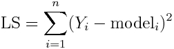
To find better values of the model parameters, I could just try lots of different values of the time of introduction, t0, and R0, and rerun the fit_example.R script many times to see whether I get a better fit or not.  Take a look at the plot below… does it look like a better fit?  Is the least squares statistic smaller?  Note that fiddling around with the model parameters by hand to find a “reasonable” fit is actually fairly often done when people are just trying to get ballpark estimates of their parameters.  It isn’t a rigorous way to do it, though.

 

 

Here is an R Shiny visual analytics app I have made for this data that has slider bars that allows the user to select the value of R0 and the time-of-introduction of the virus, and then shows the resulting SIR model prediction overlaid on the data.  The app also shows the value of the Least Squares statistic comparing the data to the model (note that the app is best viewed on the shinyapps.io server):

 

Finding the model parameters that minimize the Least Squares statistic:   why we can’t just use linear regression methods for the dynamic models we often use in applied mathematics for the life and social sciences? 

 Many readers of this module perhaps have taken an introductory statistics course, and learned about linear regression (which, as it happens, usually uses Least Squares as its figure-of-merit statistic).  All statistical/numerical interactive programming packages (ie; Matlab, R, Stata, SAS, SPSS) have in-built functions for linear regression.  Why can’t we just use those functions to estimate our model parameters?  Well…

1. Disease and population biology models that we use in our field are often non-linear.  In fact they are often very, very non-linear. “Linear” regression requires a linear model.
2. Unlike y = mx+b, the equations describing the compartmental models we use usually have no analytic solution.  They must be solved numerically using algorithms like Euler’s method, or the Runge-Kutta method.  This is computationally intensive, and in-built linear regression functions (or other optimization methods) that also have computational overhead simply cannot handle the additional underlying computational complexity, round off errors, etc, that we have to face when numerically solving the models we use.
3. With our models, our data are often just partial observations; for instance, with an SIR model, public health officials do not get simultaneous observations of S, I, and R during the epidemic.  Unless they are doing repeated seroprevalence studies over time, public health officials don’t even get estimates of I.  What they usually measure is the incidence of the disease (which, for an SIR model, is equal to beta*S*I*delta_time, where delta_time is the time step over which the incidence is measured).  Based on our SIR model and our incomplete data, we try to estimate beta.

However, despite all these complications, all is not lost!  Given enough computing power, one can readily estimate model parameters with methods known as Latin Hypercube and random sampling (Monte Carlo parameter sweeps).  All major research universities (including ASU) have high performance computing facilities, where you can run many programs in parallel on hundreds of processors at once.

There are other methods that can be used for parameter optimization (like gradient descent and simplex methods) that I’ll talk about in a later module.  As we will discuss then, in practice they don’t work well (ie; or often at all, for that matter) for the kind of parameter optimization problems we encounter with models we use in this field.  This is why I’m just skipping first to describing the method that always works…

In the example below, I talk about fitting the parameters of a simple SIR model to influenza data by finding the minimum of the Least Squares statistic by randomly sampling many hypotheses of the model parameters, and then plotting the Least Squares statistic versus the  parameter hypotheses to see which minimise the LS statistic.

The data could be from a different disease appropriate to an SIR model, or the model could be a description of any dynamic process, like animal population dynamics for instance, with data that is appropriate to the model.  So, keep in mind that I give a specific example here, but the method itself is very general and can be applied to an almost infinite variety of problems.

Graphical Monte Carlo method

Regardless of the compartmental model you are trying to fit the parameters for, or the data you are fitting, or the computer language you are using to do the fitting (R, Matlab, C++, Python, etc), the algorithm behind the Graphical Monte Carlo parameter sweep method is the same; you do many iterations where within each iteration you randomly sample hypotheses for the parameters from uniform distributions with appropriate ranges that you suspect are probably in the ballpark of what the true value of the parameter.  Then, for each of those sets of parameters you calculate your model estimate of the data distribution, and compare it to see if it is a good fit.  This isn’t just done by looking at it and thinking “Yeah, that looks like the best fit so far…”.  Instead, there are well defined quantities (“figure of merit statistics”) that you can calculate that give an indication of how well the model fits the data.  In this module we are discussing the Least Squares statistic, which, as we will discuss below, isn’t appropriate to all data types.  In later modules we will discuss other figure of merit statistics, like Poisson likelihood, and weighted (Pearson) least squares.

R code to fit SIR model to 2007-2008 confirmed influenza cases in Midwest

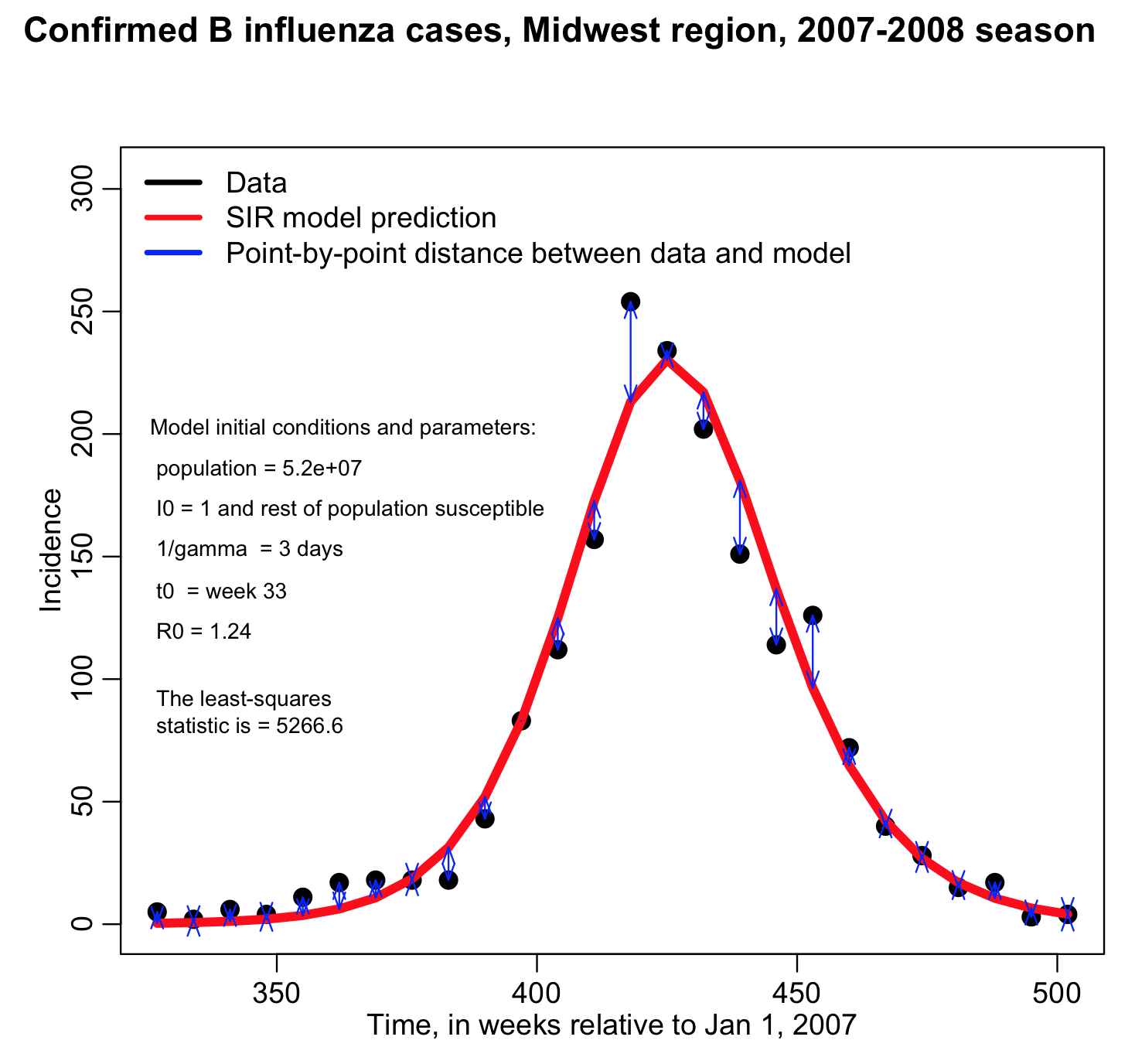
Rather than changing R0 and t0, and re-running the fit_example.R script many different times, it is much easier to write an R script to do a loop where it samples many different hypotheses for R0 and t0 and calculates the least-squares statistic, keeping track of how the least squares statistic depends on R0 and t0.

In blue I show the value of (R0,t0) that minimizes the Least Squares statistic, and then in the lower plot I overlay the best fit curve on the data.  The fit looks quite reasonable.

In the file  fit_iteration.R I provide the code that (eventually, after running a while) produces the above plots.  Note that when you try this code out it will run slowly.  This is because many, many different combinations of R0 and t0 had to be tried to get a good number of points in the plots, and a reasonable idea of what R0, t0 values will provide the best fit.  The more parameters you fit for, the more parameter combinations you will have to try to populate plots like the ones above.  In fact, the complexity of the process rises exponentially in the number of parameters.

This makes the R programming environment very non-ideal for such operations because R is not compiled; because it has a command-line interface, it waits for the next command for you to type in (or enter from a file).  This makes R very non-optimal for any process that requires many, many iterations that involve intense calculations at each iteration (which is true here, and also in stochastic modelling methods).  Thus, while R is perfectly good for examining the algorithms involved for fitting to data for instructive purposes, in a real-life analysis situation I implement the algorithm in a compiled programming language like C++ or Java, and I submit the program in batch, a thousand runs at a time, to a super computing platform.

You might be wondering how I knew what ranges to use for the Monte Carlo parameter sampling; at first I didn’t.  I did some preliminary sweeps, and made sure that the ranges I was using appeared to contain the values that minimized the LS statistic.  Then I narrowed in on that sweet spot, and did what I sometimes refer to as a “higher statistics run” (ie; a ran the script long enough that there were enough points on that plot that it was quite clear what parameter values minimized our LS statistic).

Parameter estimates have uncertainties

Did you notice above that the LS vs parameter plots have a parabolic envelope? The width of that parabola defines the parameter uncertainties (if it is a really wide parabola, you have large uncertainty for that parameter).  I won’t go into yet how exactly to calculate the parameter uncertainties from those parabolas… that will come in a later module.

But it needs to be pointed out that whatever optimization method or figure-of-merit statistic one uses when estimating model parameters, the parameter estimates will have uncertainties associated with them due to the stochasticity in the data, like migration into and out of the population, Binomial uncertainty on the number of identified cases, etc; that is to say, you don’t get an exact estimate of the model parameter.

Potential pitfalls of using the Least Squares statistic

There is a potential pitfall with fitting with Least Squares; the method carries the underlying assumption that each data point has exactly the same amount of stochastic variation, and that the stochasticity is Normally distributed.  In reality, this is usually not a good assumption for epidemic count data, where points on the initial rise and end of the epidemic curve will tend to have much more relative stochasticity than points near the peak (and may in fact have stochasticity that is not even remotely close to being Normally distributed).  It is for this reason that I don’t usually use Least Squares to fit models to epidemic curves, and instead use a method like Pearson chi-squared or Poisson or Negative Binomial maximum likelihood (talked about in other modules on this site).  When data violate the equal stochasticity assumption and/or Normality assumption, the Least Squares method can result in biased model parameter estimates.

The Least Squares method also assumes that all the stochasticity in the data are independent from point-to-point.  This is more or less true when you have a time series of incidence data.  It generally isn’t true if you have a time series of population size (for instance, the population at the next time step is quite correlated to the population at the time step before… as soon as data points are correlated, they are not independent). For population data, it is better to fit to the change in population size from time step to time step, which should result in data that are more independent from point to point. Cumulative incidence data are also not independent… the data at the next time step is equal to the cumulative data at the last time step plus a little bit more… those two data points are highly correlated.  Never use Least Squares methods to fit to cumulative incidence data. All standard fitting methods, in fact, have as an underlying assumption that the data are independent. So, as a general rule, don’t fit to cumulative incidence data at all.

I’m not going to discuss in this module the estimation of model parameter uncertainties with the Least Squares method, because it is beyond the scope of what I want to talk about here.  If you want more information on that see here, and here.  Be aware that violations of the underlying equal stochasticity assumption of least squares can not only can bias the parameter estimates, but also produce inefficient estimates of the parameter uncertainties; the estimated confidence intervals will be wrong.

If you would like to learn more about the underlying assumptions of the Least Squares method, see this module.

Things to try

Try finding some data for a different epidemic of an infectious disease (it needn’t be flu data) and fit for the R0 of the epidemic with a compartmental disease model appropriate for that disease (SEIR, SIR, SIS, SIRS, etc).  Does the R0 that you get match the R0 for the disease that you find when doing literature searches in Google Scholar?