[This presentation discusses methods commonly used to optimize the parameters of a mathematical model for population or disease dynamics to pertinent data.  Parameter optimization of such models is complicated by the fact that usually they have no analytic solution, but instead must be solved numerically. Choice of an appropriate “goodness of fit” statistic will be discussed, as will the benefits and drawbacks of various fitting methods such as gradient descent, Markov Chain Monte Carlo, and Latin Hypercube and random sampling.  An example of the application of the some of the methods using simulated data from a simple model for the incidence of a disease in a human population will be presented]

• Introduction
• Some simulated disease data in a human population
• Things to keep in mind when embarking on model parameter optimization
• Choice of an appropriate goodness of fit statistic                            
  
  • Least Squares
  • Poisson likelihood
  • Negative Binomial likelihood
  • Binomial likelihood
• Parameter optimization methods to optimize the goodness-of-fit statistic             
  
  • Gradient descent
  • Simplex method
  • Markov Chain Monte Carlo
  • Graphical Monte Carlo: Latin hypercube sampling
  • Graphical Monte Carlo: uniform random sampling

Introduction

Many of the parameters for models of the spread of disease or biological population dynamics are usually well known from prior observational studies.  For diseases like dengue and malaria, for instance, the vector population dynamics have been extensively studied in the laboratory and in the field. For diseases like measles and human seasonal  influenza, the latent and infectious period are fairly well known from observational studies.  However, for influenza, it is apparent that seasonal forcing plays a role in either the transmission and/or susceptibility, but it is currently unknown how much of this is due to climate and how much is due to seasonal patterns in human contact rates.  A model for the spread of influenza could include parameters that account for both of these effects, and these parameters can be estimated by fitting the model to seasonal influenza data.

Often times there are model parameters which must be estimated because prior knowledge is sketchy or non-existent.  An example of such a parameter is the vector/host biting rate in models for diseases like dengue, malaria, or leishmaniasis.  In addition, for newly emerged disease outbreaks (for instance Ebola), the reproduction number is not well known.

In order to accurately forecast the progression of an epidemic and/or examine the efficacy of control strategies to improve the current situation, it is necessary to have a model with parameters that have been optimized to describe current data. But in the mathematical life sciences, a hugely complicating factor in estimating model parameters is that the mathematical model itself often has no analytic solution, but rather must be solved numerically.  In addition, another problem is that our mathematical models typically are only an approximation to the actual dynamics.  This means that common regression methods coded up in platforms like Matlab or R simply will not work for these applications due to these computational complexities and model pathologies.  In this presentation, I’ll thus discuss the applicability of various methods for model parameter estimation in mathematical life sciences.

Some simulated data for a hypothetical epidemic in humans

For this presentation, we’ll use as example “data” a simulated pandemic flu like illness in spreading in a population, with true model:

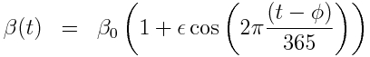
with seasonal transmission rate

The R script sir_harm_sde.R uses the above model with parameters 1/gamma=3 days, beta_0=0.5, epsilon=0.3, and phi=0.  One infected person is assumed to be introduced to an entirely susceptible population of 10 million on day 60, and only 1/5000 cases is assumed to be counted (this is actually the approximate number of flu cases that are typically detected by surveillance networks in the US).  The script uses Stochastic Differential Equations to simulate the outbreak with population stochasticity, then additionally simulates the fact that the surveillance system on average only catches 1/5000 cases.

The script produces the following plot:

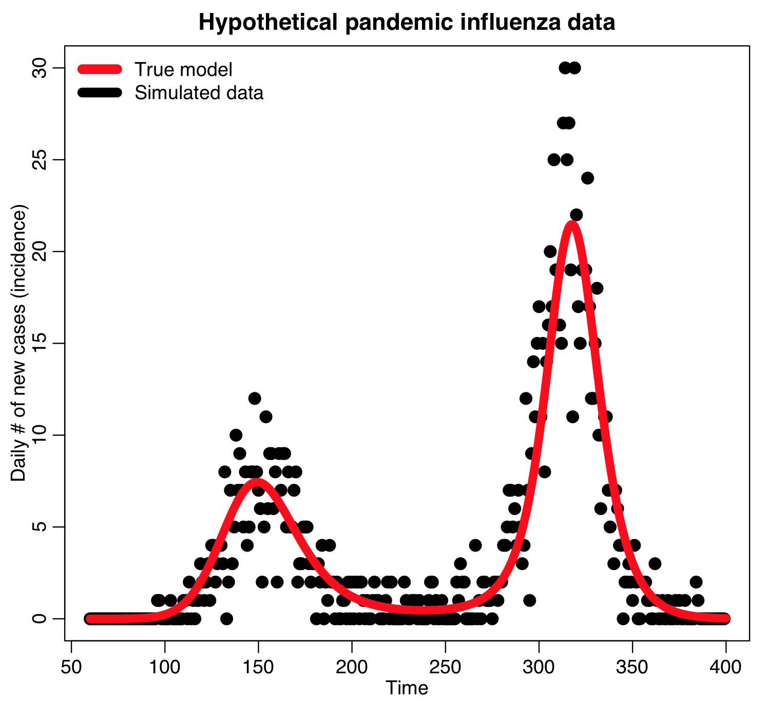
The script outputs the simulated data to the file sir_harmonic_sde_simulated_outbreak.csv

We will be using this simulated data in our fitting examples below.

Things to keep in mind when embarking on model parameter optimization

Successfully obtaining a model that is parameterized to optimally describe vector borne disease data first and foremost requires choosing a model that appropriately describes the dynamics underlying the patterns in the data.  This requires, at the very least, a knowledge of the biology of the vector population, and the epidemiology of the disease (ie; mechanism for spread, whether recovery confers immunity, etc).

We need to obtain the most parsimonious model that incorporates the most relevant dynamics.  If a model has too many parameters, even the most sophisticated of parameter optimization methods will fail!

The next step, after choosing a model, is to choose a “goodness-of-fit” statistic that will give an indication of how well a particular model parameterization is describing the data. This depends on the probability distribution that underlies the randomness in the data (more on that in a moment). Once we have that goodness-of-fit statistic, there are a variety of methods that can be used to find the parameters that optimize that statistic.

Note that the parameter estimates returned by model optimization are just that; estimates.  Because of the randomness inherent in the data, there is stochasticity inherent to the parameter estimate.  Parameter estimation not only involves estimating the best-fit parameters, but also the uncertainty on the parameter estimates (often expressed as a 95% CI).

Choice of an appropriate “goodness of fit statistic”

Optimization of model parameters involves first choosing a “goodness-of-fit” statistic (aka: “figure of merit” statistic) that depends on the data and the model calculated under some hypothesis of the parameters.  The model parameter combination that minimizes this statistic is the “best-fit” combination.  The choice of the “goodness-of-fit” statistic critically depends on the probability distribution that underlies the stochasticity in the data.

Note that because of inherent stochasticity (randomness) in population or disease count data, even a best-fit model will not perfectly describe the data.  Stochasticity in the data can be due to a wide variety of things, like randomness in population movements or contacts, randomness in births or deaths, randomness in disease case identification (not all cases of many diseases are caught by surveillance systems), etc.

There are many different goodness-of-fit statistics that can be used; choosing the most appropriate goodness-of-fit statistic involves being aware of what probability distribution likely underlies the stochasticity in the data.  Choosing the wrong goodness-of-fit statistic leads to biases in your fit results, and wrong estimates of the uncertainties in those estimates.

Some commonly used goodness-of-fit statistics (this isn’t an exhaustive list):

• Least squares and generalized least squares: appropriate for empirical data with Normally distributed stochasticity.  While you might see it often (completely inappropriately) applied to count data, this is not usually appropriate for such data.  Count data, particularly with low numbers of counts, are very non-Normally distributed and also heteroscedastic (Least Squares assumes homoscedasticity of data). Why is Least Squares so often mis-applied?  Because it’s usually the only goodness-of-fit statistic people are exposed to if they just took a Stats 101 course.  So Least Squares is most often used, but not-infrequently when it is used, it is mis-used.
• Poisson likelihood: appropriate for count data with Poisson distributed stochasticity (especially appropriate for data with few counts per unit time)
• Negative Binomial likelihood: appropriate for over-dispersed count data (ie; count data with a large amount of stochastic variation).  Nearly all count data are over-dispersed!
• Binomial likelihood (aka logistic likelihood): appropriate for data that can be expressed as k success out of N trials (ie: can be expressed as fractional data, like prevalence data)

Parameter optimization methods

A (not exhaustive) list of commonly used parameter optimization methods is as follows:

• Gradient descent: best used when a closed form solution exists for the gradient of the function to be optimized.  Algorithm is not readily parallelized.
• Simplex: No assessment of the function gradient is necessary.  Algorithm is not readily parallelized.
• Markov Chain Monte Carlo: No assessment of the function gradient is necessary.  Provides assessment of parameter posterior probability density. Algorithm is not readily parallelized.
• Graphical method: Latin hypercube sampling: No assessment of the function gradient is necessary.  Provides assessment of parameter posterior probability density. Easy to apply Bayesian priors for other model parameters. Not easily parallelized, but possible.
• Graphical Monte Carlo method: Uniform random sampling: No assessment of the function gradient is necessary.  Provides assessment of the parameter posterior probability density.  Algorithm is easily parallelized to use high performance distributed computing resources, like XSEDE, or using R with the ASU Agave cluster.  Easy to apply Bayesian priors for other model parameters.