[This is part of a series of modules on optimization methods]
As we described in this module, gradient descent methods are commonly used to find the minimum of multivariate functions (for instance, the goodness-of-fit statistic, which depends on the model, and its parameters, and the data), but have limited applicability to model parameter fitting in mathematical epidemiology/biology due to the necessity of calculating the gradient at each step in the algorithm.
Simplex methods are an alternative optimization method for goodness-of-fit statistics that do not require calculation of a gradient, just the GoF statistic itself.
Here is a (rather overly simplified) example of how the simplex algorithm works:
If you are trying to optimize k parameters, randomly pick k+1 different sets of the model parameter hypotheses, and calculate the GoF statistic, S, that correspond to each. Call these statistics S_i (i=1,…,k). This set of k+1 points is known as a simplex.
- Rank the S_i from smallest (best fit) to largest (worst fit)
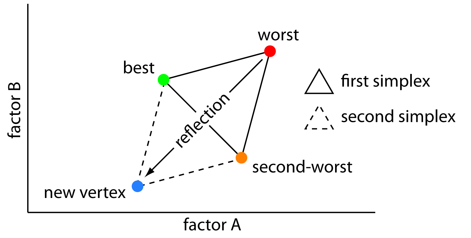
- Take the centroid of parameters corresponding to all but the largest of the S_i.
- Reflect the parameters corresponding to the largest S_i about this centroid.
- If the resulting parameters result in a new value of S that is smaller than the previous largest, then drop the previous parameters corresponding to the largest S_i and add the S corresponding to this new set of parameters to the set of k+1 GoF statistics. Go back to step 1.
- If the resulting parameters from the centroid reflection result in a new value of S that is larger than any you had at the previous step, then don’t accept this new set of parameters. Instead go back to your original step, and reflect the second worst point about the centroid of the other parameters (then third worse, etc).
- Continue until you get to a point that centroid reflection about all the k^th worst points returns an S bigger than all of them. The parameters corresponding to the smallest S are the best-fit parameters.
Here is what the first step of the algorithm looks like for two parameters:
In practice, the method is more complicated than this, employing algorithms called expansion and contraction. Nelder and Mead estimated the number of calculations needed to reach convergence as being proportional to (k+1)^22 You can see that this gets out of hand rather quickly when multiple parameters need to be estimated!
Again, this method has an advantage over gradient descent methods in that you don’t need to calculate the gradient. However, at the end you still need to estimate the Hessian in order to assess the parameter uncertainties.
The disadvantage of the simplex method applied to optimization problems in mathematical epidemiology/biology are otherwise very similar to the disadvantages associated with the gradient descent method:
- Depending on your starting guess for the parameters, the simplex procedure can walk to a local, rather than global, minimum.
- Sometimes the procedure never converges to an answer.
- There is no good graphical way to determine that the procedure has walked to a global, rather than local, minimum in S.
- The procedure cannot be readily parallelized to use distributed computing resources to speed up the computation time.
- No good way post-hoc to all the computation to include constraints from Bayesian prior-belief on the model parameters in the analysis. You have to include the constraints right from the very beginning.

