In this module we will discuss the Markov Chain graphical Monte Carlo method for finding the best-fit parameters of a mathematical model when fitting the model predictions to a source of data.

Note that “Markov Chain” is an adjective that is applicable to a variety of contexts.  “Markov” processes assume that the predictions for the future state of a system depend solely on the current state of the system.  “Chain” means that you do many iterations of the Monte Carlo random sampling (ie: a “chain” of iterations).  In Markov Chain Monte Carlo, the distributions from which you sample depend on the current state of the system.

Markov Chain Monte Carlo methods can also be used (among other things) for stochastic compartmental modelling, but that is not what this module discusses (see here instead).  In this module we only talk about MCMC method specifically applied to parameter optimisation problems.  Much confusion often arises for graduate students when they read literature they have found that describes an analysis  employing Markov Chain methods, and they assume that it means compartmental modelling with Markov Chains.

Like the simplex method and the graphical Monte Carlo method with uniform random sampling of parameters, the Markov Chain Monte Carlo optimization method does not require the estimation of the gradient of the goodness-of-fit statistic (which depends on the model parameters), thus giving it an advantage over gradient descent methods.

MCMC methods are most readily applied when the goodness-of-fit statistic is a negative log likelihood statistic (such as the Poisson or Negative Binomial negative log likelihoods, for instance).

The basic method is pretty simple in its concept (a Metropolis algorithm):

1. Start with a guess of the parameters, theta_1
2. Calculate the likelihood for this guess, L_1
3. Now guess a second set of parameters, randomly drawn from a Normal multivariate solution centered on theta_1.  The Normal distribution is known as the proposal density, or jumping distribution. With Gibbs sampling, the Normal sampling distributions for each of the parameters are assumed to be independent. The new set of sampled parameters is called theta_2.  Calculate likelihood, L_2.
4. Calculate the acceptance ratio R=L_2/L_1 (or, if negative log likelihoods are being used, calculated R=exp(neg_log_1-neg_log_2).
5. Pick a random number, r, between 0 to 1.
6. If R>r, then your new best guess is theta_1=theta_2, and go to step 3.  If R<=r then go to step 2. Using the current guess to change the sampling region is why this is a Markov Chain Monte Carlo method (Markov Chain algorithms inherently choose what to do next based on the current state of the system… that’s what the adjective “Markov Chain” means).
7. The algorithm is  terminated after some fixed (large) number of iterations. The distributions of the accepted values of the parameters at the various iterations forms what is known as the “posterior probability distributions” of the parameters

Note that in step 6 that if L_2>=L_1 (ie; the negative log likehood with theta_2 is smaller than the negative log likelihood with theta_1) we will always accept theta_2 as the new best guess. However, if L_2<L_1, we will sometimes reject the move to theta_2 as the new best guess, and the more the relative drop in likelihood, the more probable we are to reject the new point. Thus, we will tend to stay in (and return large numbers of samples from) high-density regions of the likelihood (ie: the probability distribution for theta) while only occasionally visiting low-density regions.

Note that the parameters of the Normal sampling distribution depend only on your current best-guess (ie; the current state of the system): this is what makes this a Markov Chain Monte Carlo process.

The complicated part about this method is choosing the multivariate widths of the Normal distributions used in step 3.  Too narrow, and you are likely to get stuck in local minima, and/or the algorithm takes a long time to walk to the minimum because the steps are too tiny.  Too broad, and you waste a lot of time evaluating points that are nowhere near the global minimum.  In practice, the widths of the multivariate Normal distribution are tuned during the initial iterations, known as the burn-in period.  The more parameters that must be optimized, the longer the burn-in period.

The advantage of this method is that you can readily get a posterior probability density for the model parameters just from the distribution of the chosen values at each step.

A primary disadvantage is that, just like the simplex and gradient descent methods, the method is prone to walking towards local minima.  And you would never know simply by plotting the negative log-likelihood versus your sampled parameter hypotheses, because the parameter hypotheses will be preferentially sampled in the region of that local minimum.

One problem with the MCMC method is that it is computationally clunky to include the effect of uncertainties on other parameters in the model.  If another parameter of the model has some uncertainty associated with it (because, for example, it is not perfectly known from either experiment or observational studies), that uncertainty has some probability distribution associated with it (aka: a Bayesian prior probability distribution). If what we see quoted in the literature is a mean and one standard deviation uncertainty, we usually assume the Bayesian prior distribution is Normal with that mean and one std deviation variation.  For example, we don’t know the recovery period of influenza, 1/gamma, perfectly from observational studies, but most studies agree that it appears to be somewhere in the range 2 to 5 days.  In this case, our Bayesian prior probability distribution for 1/gamma would be Normal, with mean around 3.5 days and std deviation width around 1 day.

Unfortunately, unlike with uniform random sampling of parameters, you cannot readily apply Bayesian parameter prior-belief distributions in a post-hoc way to constrain the posterior probability distributions of the parameters you are fitting for in the MCMC method (you have to include the Bayesian priors in the likelihood right from the very start).  Here is a module which discusses including Bayesian priors when using uniform random sampling for the parameter hypotheses 

Example: fitting parameters of a harmonic SIR model to simulated pandemic influenza data

Here we will examine simulated data for a hypothetical pandemic influenza outbreak.

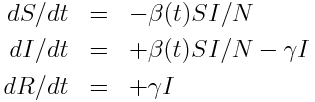
Recall that the model equations for a disease with seasonal transmission are:

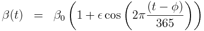
with harmonic transmission rate:

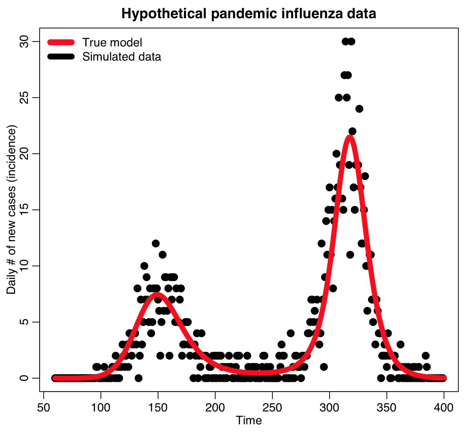
Using Stochastic Differential Equations, the sir_harm_sde.R script simulates an epidemic in a population with 10 million and with one infected person introduced to an entirely susceptible population.  In addition to the effects of population stochasticity, the script also simulates a surveillance system that only records on average 1/5000 cases.  The script assumes R0=beta0/gamma=1.5, phi=0 (the day of year, relative to Jan 1st that the virus is most transmissible), time of introduction t0=day 60, and epsilon=0.30.

The simulated data look like this, and can be found in the file sir_harmonic_sde_simulated_outbreak.csv:  

Fitting to the data

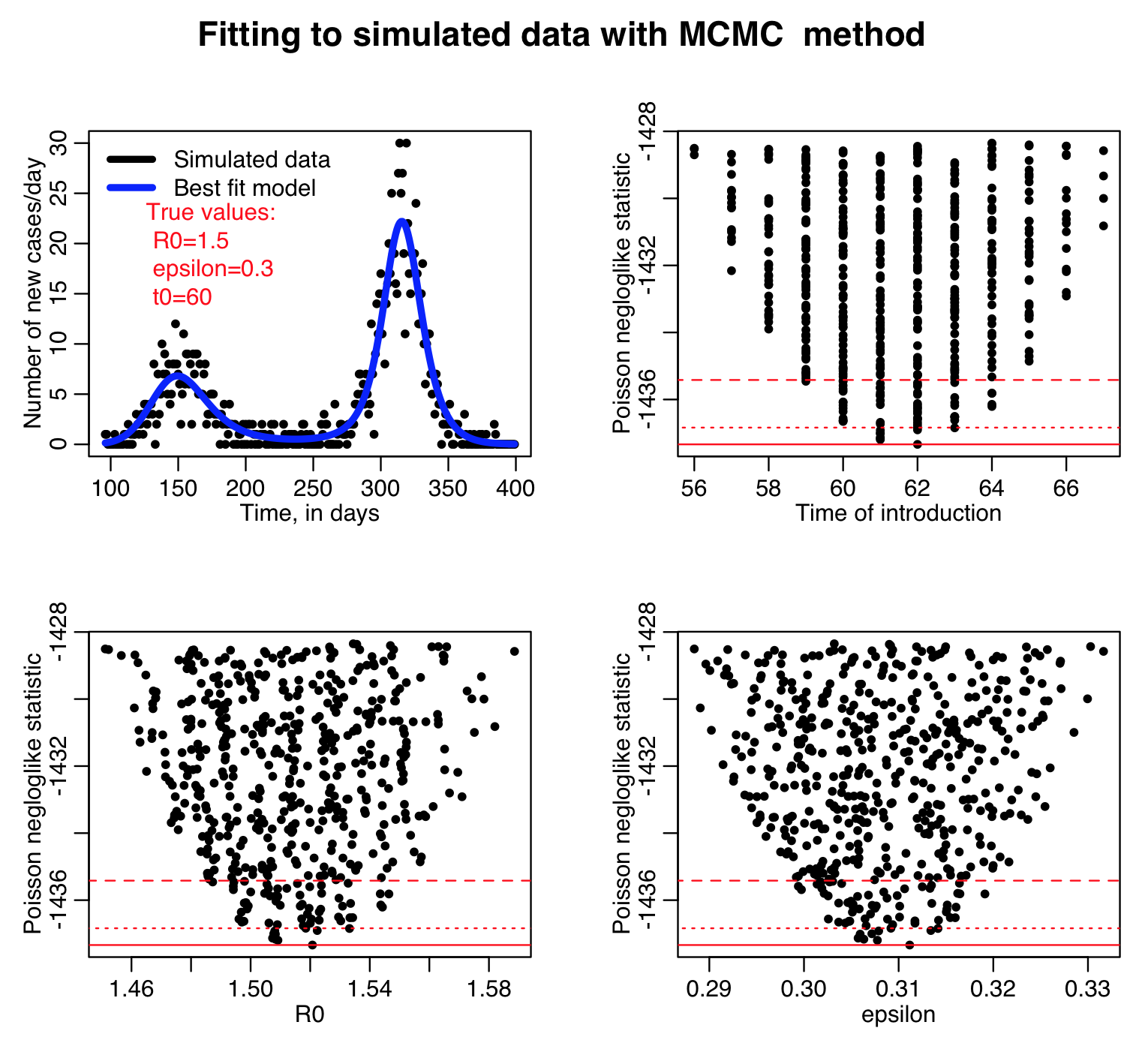
The R script sir_harm_mcmc_fit.R applies a rudimentary MCMC method to optimize the parameters of a harmonic SIR model to the simulated pandemic influenza incidence data.

In the algorithm, we use Poisson negative log likelihood as the goodness-of-fit statistic.

Here is the result of running the sir_harm_mcmc_fit.R script for 100000 iterations, sampling R0, the time of introduction t0, and epsilon parameters of our harmonic SIR model over certain ranges (how did I know which ranges to use? I ran the script a couple of times and fine-tuned the parameter ranges to ensure that the ranges actually contained the values that minimized the GoF statistic, and that the ranges weren’t so broad that I would have to run the script for ages to determine a fair approximation of the best-fit values).  Do you think 100000 iterations is enough?

This was a rudimentary implementation of the MCMC algorithm in that I did not re-assess the sampling ranges after a burn-in period.  What I should have done, after several thousand iterations, is to find the average values of the sampled values, and their one std deviation variation, and then begin sampling from Normal distributions with those properties instead.