In another module on this site I describe how an epidemic for certain kinds of infectious diseases (like influenza) can be modelled with a simple Susceptible, Infectious, Recovered (SIR) model. Readers who have not yet been exposed to calculus (such as junior or senior high school students) may have been daunted by the system of differential equations shown in that post.  However, with only a small amount of programming experience in R, students without calculus can still easily model epidemics, or any other system that can be described with a compartmental model.  In this post I will show how that is done.

Modelling an epidemic using small time steps in the simulation

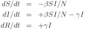
First read the previous module, concentrating on the description of the how disease spreads in the population, rather than the equations of the SIR model.  In the post, I describe how the SIR model is a compartmental model, with flow out of the susceptible compartment and into the infected compartment equal to beta*S*I/N, where beta is known as the transmission rate, and S and I are the number of susceptible and infected in the population at some point in time.  The flow out of the infected compartment and into the recovered compartment is gamma*I, where gamma is the recovery rate.  The compartmental diagram for the model is:

and the differential equations describing this model are

If we look at a very small time step (say, delta_t=0.10 days or even smaller), we can approximate those derivatives on the left hand side by expressing them instead as a small change in S (for instance) divided by the small change in t.

The small change in S and I during each small time step, delta_t, will thus be

delta_S = -(beta*S*I/N)*delta_t 
delta_I = (beta*S*I-gamma*I)*delta_t

We thus start the simulation with S=N-1, and I=1 (N is the population size) and move through time in little time steps delta_t, and at each time step incrementing S and I as follows:

S_new = S_old - (beta*S_old*I_old/N)*delta_t 
I_new = I_old + (beta*S_old*I_old/N-gamma*I_old)*delta_t

Where S_old and I_old are the values of S and I at the previous time step.  Note that delta_S=(S_new-S_old) and delta_I=(I_new-I_old)… that’s how I derived the expressions for S_new and I_new from the expressions for delta_S and delta_I above.

In the simulations, we just keep on stepping through time, until we get to the point where I_new is less than or equal to zero, at which point the epidemic has ended.  Or until we want to end the simulation after a certain number of time steps.  Whichever.

In the file sir_without_calculus.R I show how to implement this algorithm in R.  To make the plots that the script produces look nice, I used a function in the R sfsmisc library.  To install sfsmisc in R type in the R command line:

install.packages("sfsmisc")

Choose a mirror site somewhere in the world close to you.  It doesn’t really matter which you pick (but if you pick one far away the installation will be slower).

To run sir_without_calculus.R first download the file.

Note to Windows users: ensure that Windows doesn’t sneakily append “.txt” to the end of the file, otherwise the instructions below will not work (ie; don’t save it as a text file in Windows, otherwise Windows adds a hidden “.txt” at the end of the file name). 

Also, for users of all operating systems, save the file with the name exactly as I have it here.

Now take a moment to read through the file.  It is heavily commented and should be fairly self-explanatory. Then, in the R console window type

source("sir_without_calculus.R")

making sure that R is in the same working directory as the file by first typing

setwd("<the pathname of directory containing the file">)

If you have problems setting the working directory in the Windows operating system, the problem could be in how directory paths are written in R: make sure you use forward slashes in the directory path name, instead of the backward slash you are used to using in Windows.  So, an example of using setwd in R running in Windows is setwd(“C:/Users/mydirectory/”)

The following plot should be produced:

The method I show here is often referred to as a simple time-difference method (because of the small time steps), or Euler’s method.  Using time-difference methods to numerically solve systems of ODE’s that are associated with compartmental models is intuitively pretty simple (so simple that I’ve seen a 12 year old do it).  Using compartmental models to describe things like epidemics or predator/prey systems could potentially make an interesting science fair project.  There are a lot of things that can be described with compartmental models. Even the spread of ideas.

The importance of using a small time step

When using time-difference methods to simulate compartmental models, you have to be very careful to ensure delta_t is small. If it is too big, then the change in the compartments from step to step will also be big, and this computational algorithm for modelling the epidemic will no longer work properly.  I’ve found that 0.10 days is usually sufficient for SIR modelling of influenza epidemics in modest population sizes, but the appropriate time step really depends on what you are trying to model, and how big the population size (for big populations, to get a good approximate solution you need even smaller time steps).

To double-check your time step is small enough, halve it and ensure that the simulation returns the same epidemic curve (and if it doesn’t, halve the time step again and repeat the process… if it still doesn’t return the same epidemic curve as the iteration before, keep halving the time step and iterating until it does).

This issue of appropriate time step is one of the few drawbacks of doing numerical compartmental model simulation in this manner; the more sophisticated methods in the functions in the deSolve package in R internally take care of the time step issue without the user ever having to worry about it.

In the simulations presented here, we used a constant time step.  In fact, a time step that dynamically varies is best; when the number of individuals in the compartments is changing a lot (say, near the peak of an SIR epidemic), you need a smaller time step than you would need at the beginning or end of the epidemic in order to achieve good accuracy in the solution.  In another module, we discuss how to calculate the time step dynamically.