
In previous modules, we have described how to use methods in the R deSolve library to numerically solve systems of ordinary differential equations, like the SIR model. The default algorithm underlying the functions in the deSolve library is 4th order Runge-Kutta method, which involves an iterative process to obtain approximate numerical solutions to the differential equations. Euler’s method is an even simpler method that can be used to estimate solutions to ODE’s, but 4th order Runge-Kutta is a higher order method that is more precise.
Essentially these iterative numerical methods involve much the same thing: you get an estimate of the model solution at a particular time point, and then use those values to estimate the time derivatives of the compartments at that point. With the estimated derivatives, you thus know how much the function will change if you were to take a tiny time step. So, to calculate the estimates at the next time step, take your current values plus the estimated change. Then recalculate the derivatives, estimate the change over a time step, and so on, and so on, iterating the process as long as you want.
It is important to note that Runge-Kutta and Euler methods only work properly when the time steps are *tiny*. Tiny means that the change in the compartments over that time step needs to be on the order of 1 (ie; the time step is so small that on average just one individual moves to a new compartment). In reality, in the R deSolve methods (and in Matlab ode45 methods), the methods, invisibly to you, employ dynamic time steps to solve the differential equations, where a much smaller time step is used at points when the time derivatives of the compartments are large.
For the relatively simple models that we will deal with in this course, it is enough to make sure your time step is quite small compared to the overall temporal range. For instance, for a flu epidemic that is simulated to last several months, I will often use 1/100th of a day as a time step in the simulation. As we will discuss below, when you implement the Runge-Kutta method in C++ with a constant small time step, you’ll need to double check that the answers from your program match the answers you get with the somewhat more sophisticated methods implemented in R.
A C++ class for numerically solving systems of ODE’s
In the files cpp_deSolve.h and cpp_deSolve.cpp I have written C++ code to implement the 4th order Runge Kutta method to solve systems of ODE’s. I have included example code to numerically solve the SIR and SEIR models, and a harmonic SIR model. If you want to modify this class to solve the differential equations of your own model, you need to modify the ModelEquations() method, to provide the code describing the time derivatives (very similar to what you need to do in R to use the R deSolve library).
In the file SIR_example.cpp, I give an example of an implementation of this class to numerically solve an SIR model. To compile and link the files, you can use the makefile makefile_solve by typing
make -f makefile_solve SIR_example
The program writes to standard output the temporal estimates of S and I and R. To run the file, and re-direct the results to a file called sir.out, type
./SIR_example > sir.out
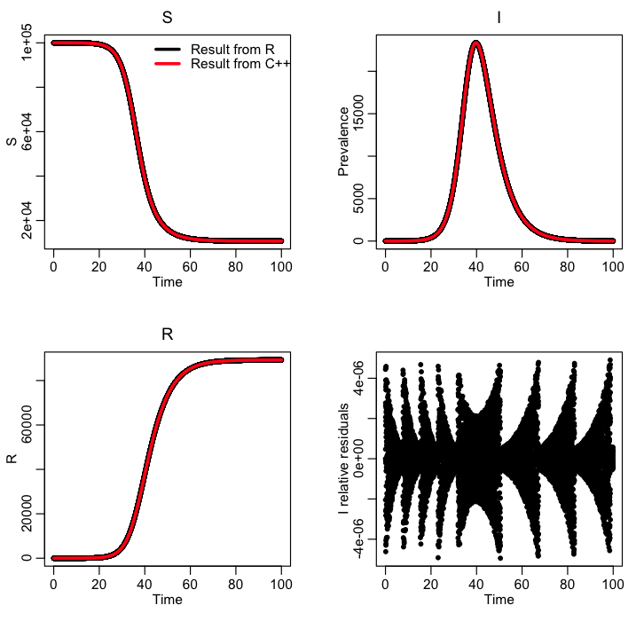
The R file SIR_example.R reads in the output file, and compares it to the results of solving the SIR model within R. The C++ results need to be very close to the R results in order for us to trust that the C++ code is doing the calculation correctly. Here is the plot produced by the R script:
Binning the output to match the temporal binning of data
When we solve a set of differential equations using either the cpp_deSolve class in C++ the time step we use necessarily needs to be tiny. However, the time step for which disease or population data are reported are typically much larger. Anywhere from a day, to a week, to a month, to a year. Thus we must bin the output of our cpp_deSolve class methods such that they match the binning of the data: once we’ve done this, we can calculate goodness-of-fit statistics, like Least Squares, Pearson chi-squared, Poisson negative log-likelihood, etc.