
[After reading this module, you will be aware of the limitations of deterministic epidemic models, like the SIR model, and understand when stochastic models are important. You will be introduced to three different methods of stochastic modelling, and understand the appropriate applications of each. By the end of this module, you will be able to implement a simple Agent Based stochastic model in R.]
Contents:
- Introduction
- Stochastic epidemic simulation: stochastic differential equations
- Stochastic epidemic simulation: Markov Chain Monte Carlo
- Stochastic epidemic simulation: Agent Base Modelling
- R function for Agent Based simulation of an SIR model
Deterministic epidemic models, like the Susceptible, Infected, Recovered (SIR) model are extraordinarily useful tools in epidemiology. Models like the SIR model can be extended to include heterogeneity of transmission (like different transmission rates for different age classes, time dependent transmission, etc), and heterogeneity of the population (like age structure, gender structure, etc). Compartments that describe isolated, quarantined, or vaccinated individuals can be added, and deaths and births can also be included.
Numerical solution of deterministic models with modern computers is almost instantaneous, and these models thus lend themselves well to studies that lead to optimized disease intervention strategies, such as vaccination programs targeted at segments of the population that tend to be super-spreaders of disease.
However, despite the many advantages of deterministic models, it can be difficult (but not impossible) to include realistic population networks (like family, school, and workplace networks) in such models. It can also be difficult to incorporate realistic probability distributions for the time spent in the infectious period. Deterministic models also do not allow us to assess the probability of an outbreak, and the probability distributions of the final size of an epidemic in small populations.
Stochastic epidemic simulation: stochastic differential equations
There are several ways to stochastically simulate epidemics. Models based on stochastic differential equations (SDE’s) are very similar to ODE deterministic models, except that the time derivatives of the compartments include an extra stochastic term. SDE’s have the advantage that, computationally, the simulation runs almost as fast as that of the equivalent deterministic ODE model. SDE’s have the disadvantage that the stochastic term sometimes results in the number of susceptibles in the population going up (which is technically impossible, in the absence of births or recurring susceptibility after recovery). SDE’s are also just as limited as ODE’s at describing networked populations and other heterogeneities that are important to the dynamics of disease transmission. However, tor medium to large populations SDE’s work quite well for quick assessment the probability of outbreak and/or the probability distribution of the final size of the epidemic. I will likely discuss epidemic modelling with SDE’s in much greater detail at a future date, and provide R scripts for SIR modelling with SDE’s.
Stochastic epidemic simulation: Markov Chain Monte Carlo
For small populations, Markov Chain Monte Carlo (MCMC) methods are useful for stochastic simulation. MCMC methods step through the simulation in very tiny time steps… so tiny that only one “event” happens on average during that step (where an “event” could be an infected person recovering, or a susceptible person getting infected). At each time step the probability of each possible “event” is assessed, and one of the events is chosen randomly (weighted by its probability of occurrence). A nice thing about MCMC is that if the population and disease spread dynamics are such that the number of susceptibles always should go down (or stay the same), MCMC methods ensure that occurs. MCMC methods are thus useful for simulating the spread of disease in small populations. The disadvantage of using MCMC methods for epidemic modelling is that they can be somewhat slow because of the tiny time steps. Also, MCMC can be just as limited as SDE’s and ODE’s when it comes to incorporating networked populations and other heterogeneities.
At a future date, I will likely write in detail about MCMC epidemic simulation methods, and provide R scripts for SIR modelling with MCMC.
Stochastic epidemic simulation: Agent Based Modelling
The final method of stochastic epidemic simulation that I will discuss here is Agent Based Models (ABM), also known as Individual Based Models (IBM). ABM’s have the advantage that you can put all kinds of detail into the model at the individual level (ie; you can set up your population, give them different ages, have people living in households with other people, going to school/work with other people, etc). You can also implement arbitrarily complex probability distributions for the time spent in the infectious period, etc.
Because of the almost infinite complexities that can be incorporated into an ABM, they can be very, very slow to simulate epidemics in populations of even moderate size (like a town). A potential pitfall of using ABM’s is that it can be all too easy to get carried away with model complexity, resulting in lots of model parameters, especially if you have to start guessing the values of various parameters because little data exists to indicate what the true values should be. There is a saying called GIGO (“garbage in, garbage out”) that can well apply to ABM simulations that have too many arbitrarily chosen parameters. Because of the GIGO pitfall, I always ask myself if I really need to perform a simulation with all that complexity to answer a particular research question (the answer is often “no”, and I turn to a method like SDE’s or MCMC instead).
The fun thing about ABM’s is that in addition to allowing a lot of freedom in complexity of simulation, they are, well… fun. Setting up your population, then introducing a disease and watching what happens is kind of like playing Sims.
R function for Agent Based simulation of an SIR model
In the script sir_agent_func.R I provide a function for Agent Based modelling of a SIR epidemic in R. While it is perhaps instructive to do your first attempt at ABM with this script (because you can compare it to the deterministic SIR model results), be aware this is probably one of the most inappropriate implementations of ABM possible… the population is homogeneously mixing and there is no individual level structure at all! Running this particular script is thus a bit of a waste of good CPU cycles that would be better applied to doing the same thing with an MCMC simulation (but I haven’t talked about how to implement MCMC yet, so for now we will just talk about ABM’s).
The function in sir_agent_func.R takes as arguments the population size, the initial number infected and susceptible in the population, the rate of recovery, the reproduction number, and the start and end time of the simulation, with some time step delta_t.
The simulation begins by setting up “state” vectors for each individual in the population. This vector records the state of the individual (0 if susceptible, 1 if infected, and 2 if recovered). Initially, most of the population is susceptible with just a few infected people.
If an individual is infected, the SIR model has as an inherent underlying assumption that the time spent in the infectious period is exponentially distributed. The probability that an infected individual recovers in time step t to t+delta_t can be shown to be
1-exp(-gamma*delta_t)
where gamma is the recovery rate. In addition, in an SIR model scenario, a susceptible person contacts a Poisson distributed random number of people in each time step, with average beta*delta_t*I/N, where beta is the transmission rate.
Given values of S and I at a particular time step, we thus stochastically simulate the number of infected people that each S contacts in that time step by randomly sampling the Poisson distribution. If the number of contacts with infectives is greater than 0, we change the state of the susceptible person to “infected”.
For each infected person, we draw a random number between 0 and 1 from the uniform distribution. If this number is less than 1-exp(-gamma*delta_t), we change the individual’s state to “recovered”.
The simulation in the function steps through time in this manner, stopping when there are no more infectious people, or when we reach a maximum time end point.
R program for Agent Based Modelling
The file sir_agent.R calls the function in sir_agent_func.R in order to stochastically simulate an influenza epidemic under the assumption that the population mixes homogeneously. To run the program, download both files to your working directory in R (and make sure the odesolve package has already been installed). Then type
source("sir_agent.R").
The simulation will take a bit of time to run because it does 25 simulations, and produces the following plot
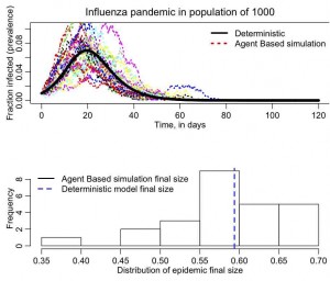
(your plot may differ a bit because your random seed is different than mine).
R program for Agent Based Model with population structure
In agent_grid.R I provide an R script that puts individuals in a population on a grid, and only allows the individuals to infect their neighbors on the grid. The script plots the grid at each time step, showing with different colors the population members that are susceptible (grey), infected(red), or recovered (blue). There is no random mixing in this population, and at each time step the script picks a number of neighbors that each infective contacts from the Poisson distribution (take a look at the code; what do you think will happen when choosing that number if you make the time step too big?). If the infective contacts a susceptible neighbor, that neighbor changes to infected. The script also chooses a uniform random number between 0 and 1, and checks to see if that number is less than the probability of recovery. If true, then the individual recovers. The simulation continues, stepping through in small time steps, and stops when there are no more infected people in the population.
Things to try
Time how long the sir_agent.R script takes to run. Now increase the population in the simulation by a factor of 10. How much longer does the script now take to run?
Notice that the time step I used in the simulations is delta_t=0.1 days. See what happens when you change this to a large time step (say, 10 days). Do you think the result is a realistic simulation of disease spread in the population? (hint: the time step should be small enough that the change in S and/or I in that time step is small).