[After going through this module, students will be familiar with time-dependent transmission rates in a compartmental SIR model, will have explored some of  the complex dynamics that can be created when the transmission is not constant, and will understand applications to the modelling of influenza pandemics.]

Contents:

• Introduction
• Periodic transmission rate
• The time-of-introduction of the virus is a parameter of the model
• Some conclusions we can draw from the model
• R code for SIR model simulation with a harmonic transmission rate
• Things to try
• More things to ponder

 

Introduction

Influenza is a seasonal disease in temperate climates, usually peaking in the winter.  This implies that the transmission of influenza is greater in the winter (whether this is due to increased crowding and higher contact rates in winter, and/or due to higher transmissibility of the virus due to favorable environmental conditions in the winter is still being discussed in the literature).  What is very interesting about influenza is that sometimes summer epidemic waves can be seen with pandemic strains (followed by a larger autumn wave).  An SIR model with a constant transmission rate simply cannot replicate the annual dual wave nature of an influenza pandemic.

Periodic transmission rate

For the discussion here, we will assume that the transmission rate has annual periodicity. Any periodic function can be expressed by an infinite sum of sines and cosines, so here we will make the simplifying assumption that the transmission rate is approximated by the first order harmonic

where beta_0 is the baseline transmission rate, epsilon is the relative seasonal forcing, and phi is the day of the year when the transmission rate is maximal.

The system of differential equations for the seasonally forced SIR model are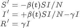
Note that, unlike the SIR model with a constant contact rate, we now have the time derivatives of S and I dependent on a function of time.  This is called a non-autonomous system of differential equations.  The mathematical analysis of non-autonomous disease models is much nastier than that of autonomous models, and the reproduction number is not straightforward to define.  In addition, there is no nice formula for the final size like we were able to derive for the autonomous model.

The time-of-introduction of the virus is a parameter of the model

In fact the final size of the epidemic whose spread is described by the above equations is a function of the start time of the epidemic, relative to the day of the year when the transmission rate is maximal (I often refer to this as the time-of-introduction of the virus to the population).  We will see in a moment that the time-of-introduction can have a profound impact on the shape of the epidemic curve and final size of the epidemic.

Some conclusions we can draw from the model

Based upon the above equations there are some interesting observations we can make:  note that maxima and minima in the the prevalence, I, occur when dI/dt=0.  From the above equations, we see that these extrema occur when S/N=gamma/beta(t).  Now we know that S is always decreasing (in a model with no births, and where recovery from infection results in immunity).  This implies that at each successive extrema in the prevalence, beta(t) must be larger than it was at the previous extrema (and this is true no matter what the time dependence of beta(t) is).  So, in the 1918 and 2009 pandemics that had summer waves, the transmission rate at the minimum in prevalence between the summer and autumn waves was greater than it was in the summer.  And the transmission rate at the peak of the autumn wave was still greater.  This observation gives at least some information about how the transmissibility of flu changes during the course of the year.

R code for SIR model simulation with harmonic transmission rate

In the file sir_harmonic.R, I provide the code that will numerically solve the differential equations above, with different times-of-introduction of the virus to the population.  First ensure that the R package deSolve has been installed in R on your computer. If it hasn’t been installed yet, in the R console, type

install.packages("deSolve")

Then download sir_harmonic.R to your R working directory, and type in the R console

source("sir_harmonic.R")

The following plot should be produced: 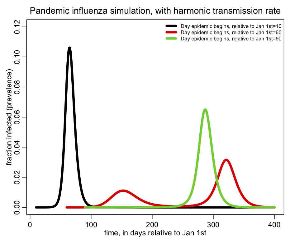You can see that the shape of the epidemic curve really depends on the time-of-introduction.  The R script also prints out the total fraction of the population that has been infected by the end of the epidemic, and you’ll notice that it too depends on the time-of-introduction.

I also show in the script a nice little trick in R to determine where local extrema occur in a time series, and in the script I used it to print out the times when the prevalence is at a minimum or maximum.

R Shiny visual analytics application for SIR modelling with harmonic transmission 

Shiny is an R package that makes it easy to build interactive web apps straight from R. You can host standalone apps on a webpage or embed them in R Markdown documents.

On the web page https://sjones.shinyapps.io/geneva you will find an R Shiny application I have written that reads daily incidence data during the 1918 influenza pandemic in Geneva, Switzerland from a file I have put in my GitHub repository.  The data are from the publication:
Chowell, G., et al. “Transmission dynamics of the great influenza pandemic of 1918 in Geneva, Switzerland: Assessing the effects of hypothetical interventions.” Journal of theoretical biology 241.2 (2006): 193-204.

The script allows the user to enter the model parameters in via slider bars, then numerically solves the SIR model with harmonic transmission with those parameters.  The resulting prediction for the daily incidence is overlaid on the data.  The page looks like this (it looks better if you go to the actual app website…):

Things to try

Edit sir_harmonic.R and examine how the final size and shape of the epidemic curve change when you change the initial number in the population that are infected, I_0.  Can you see that increasing I_0 is really pretty much the same as introducing just one infected person at an earlier time?

Try keeping the reproduction number R0=1.5, and change epsilon to 0.10.  Change the time of introduction vector, vt0, to be a wide range of values in steps of 5 days, like

vt0=seq(-180,180,5)

What times-of-introduction (if any) produce a dual wave of infection?   Repeat the process with epsilon=0.50.

Now change R0 to 1.2, and try different values of epsilon (like 0.1, 0.3, and 0.5), and a wide range of times-of-introduction to see what kind of epidemic curves you get.  Notice that for the times-of-introduction that do produce dual waves, those waves appear to occur around a year apart, just like seasonal influenza epidemics (note that several studies have estimated the relative seasonal forcing of influenza to be around 20% to 30%).

Try other types of time-dependent periodic transmission rates, and see if you can produce dual epidemic waves.  For instance, you can try a Heavyside step function that makes the transmission go down somewhat in the summer,  compared to the rest of the year (similar to what we would expect when kids go on holiday and reduce their contact rates with other kids).  To help you out, in the file heavyside.R I give a function that implements an approximation to the Heavyside step function that is differentiable (non-differentiable functions in systems of ODE’s make the problem “stiff”, and the software for numerically solving such systems will generally perform better if you remove some of the stiffness). Note that the Heavyside function I provide is also useful if you use a package like Mathematica to solve the system of ODE’s; using just a step function will cause Mathematica to choke when attempting to compute the numerical solution.

Another instructive thing to do is to edit sir_harmonic.R to print out the fraction of susceptibles in the population when the prevalence is at maxima or minima. Prove to yourself that S/N=gamma/beta at those points.

More things to ponder

There needs to be more research done on the analysis of harmonically forced SIR models.  For instance, I have used this model a lot (or modified versions of it) when modelling influenza, and one thing I have noticed is that if

epsilon=(beta_0-gamma)/beta_0=(R0-1)/R0

then there always appears to exist at least one time-of-introduction (and often many times-of-introduction) where a dual wave epidemic curve is produced (here I assume R0=beta_0/gamma).  This occurs regardless of the value of R0.  Even though I have observed this, I haven’t been able yet to mathematically *prove* that this assertion is true.

Why is this important?  Because the relative seasonal forcing of influenza has been estimated by several studies to be around 20% to 30%, and the reproduction number R0 of the 2009 influenza pandemic was estimated at the beginning to be around 1.5.  Look how closely the actual seasonal forcing of influenza matches the “sweet spot” value of epsilon that is calculated from R0!  Does this property explain why pandemic influenza is adept at producing in summer epidemic waves?

If you are able to prove the assertion above, I’d be very interested to hear about it!