
[This is part of a series of modules on optimization methods]
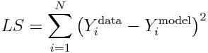
The simplest, and often used, figure of merit for goodness of fit is the Least Squares statistic (aka Residual Sum of Squares), wherein the model parameters are chosen that minimize the sum of squared differences between the model prediction and the data. For N data points, Y^data_i (where i=1,…,N), and model predictions at those points, Y^model_i, the statistic is calculated as (note that the model prediction depends on the model parameters):
Graphically, it looks like this:
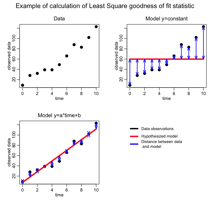
The advantage of the Least Squares statistic is that it is intuitive and easy to understand. But, it is not appropriate for all data…
Assumptions of the Least Squares statistic:
Using the Least Squares statistic in parameter optimization assumes that the stochasticity (randomness) in each data point is Normally distributed about the true model, and the Normal distribution has equal variance for each of the data points (ie; the data are “homoscedastic”). It also assumes that the stochastic variation from point to point is independent… an example of when this is (almost maximally) violated is data that are cumulatively summed. It is usually a very bad idea to fit to cumulatively summed data unless you know enough about statistics to construct a figure of merit statistic for goodness of fit that takes into account the large bin-to-bin correlations, which is a non-trivial task.
If any of these underlying assumptions are violated, the parameter optimization method can return biased estimates of the model parameters and/or incorrect assessments of the uncertainty on the parameter estimates.
When is the Least Squares method inappropriate:
Many people who use the Least Squares statistic to assess the goodness-of-fit of their model are simply looking for a simple and intuitive way to determine if their model parameters give a reasonable description of the data. If you want to be more rigorous, however, and get best estimates of the model parameters that are unbiased and have an estimate of the confidence interval (ie; the uncertainty on the parameter estimate) you need to ensure that your data comply with the underlying assumptions of whatever goodness-of-fit statistic you are using.
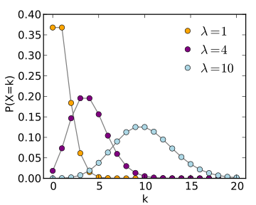
For instance, if you are fitting a model to disease or population count data where the counts are quite low (approximately less than 10), the data stochasticity is not Normally distributed, and LS is an inappropriate goodness-of-fit statistic (Poisson or Negative Binomial maximum likelihood would be a better choice). In addition, if you are fitting to count data and there is a wide variation in the number of counts, the stochasticity in the data will not be homoscedastic, and LS is again inappropriate.
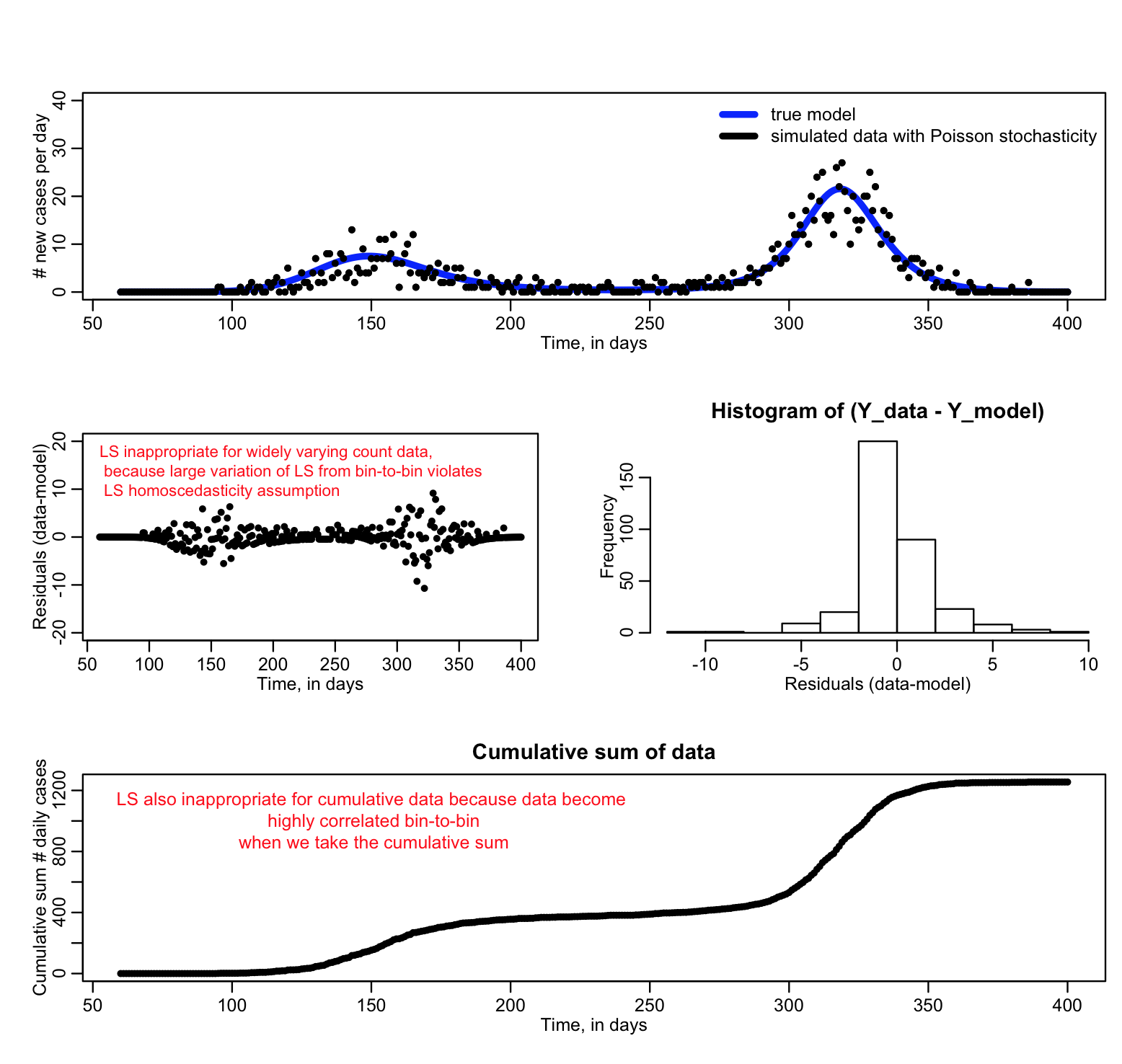
See the large variation from bin to bin in the second plot when we plot the residual squared? That’s a sign that the homoscedasticity assumption of Least Squares is being violated. If you go ahead and use Least Squares anyway, you run the risk of biased parameter estimates and you will not have a correct estimate of the uncertainty on the parameters.
If we wish to fit a model to count data, and there are at least several counts at each data point, the Least Squares method can be modified to be appropriate for widely varying data that violate the LS homoscedasticity assumption, if we use the model expectations to weight the sums of distances between the data and model expectations:
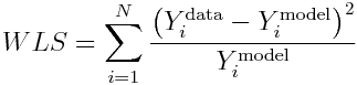
This is known as the Pearson chi-squared statistic, and is an example of a Generalized Least Squares statistic. It’s underlying premise is that the true probability distribution underlying the data stochasticity is Poisson (which approaches Normal when the counts are high enough).
Using Pearson chi^2 is much more preferable to using LS with count data. It fixes the problem we saw above with the large variation in LS from point to point (a sign that the data violate the LS homoscedasticity assumption):
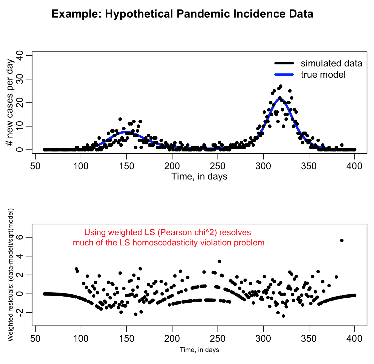
If the Pearson chi^2 is really appropriate to take into account the random variation in the data the average of (data-model)^2/model over all the bins should be around one. If it is a lot bigger than one, it is a sign that your count data are over-dispersed compared to the Poisson distribution (ie; they show more random variation than can be accounted for with Poisson stochasticity alone).
Take a look at the sir_harm_generate.R script that produced the above plots… is the mean of the Pearson chi^2 statistic for the bins approximately equal to one? ie; calculate mean(pearson_weighted_residuals^2). The simulated data were generated with the model as the expected number of counts, with Poisson random smearing… would you expect the mean of the Pearson chi^2 statistics to be one?