
In this past module, we talked about the “fmin+1/2” method that can be used to easily estimate one standard deviation confidence intervals on parameter estimates when using the graphical Monte Carlo method to fit our model parameters to data by minimizing a negative log likelihood goodness of fit statistic. In this module, we will discuss an alternate method to the fmin+1/2 method for estimating parameter uncertainties, the works for many cases, and also provides an estimate of the covariance matrix of the parameter estimates (something that is very difficult to do with the fmin+1/2 method).
As discussed in that module the model parameters can be estimated from the parameter hypothesis for which the negative log-likelihood statistic, f, is minimal, and the one standard deviation uncertainty on the parameters is obtained by looking at the range of the parameters for which the negative log likelihood is less than 1/2 more than the minimum value, like so:
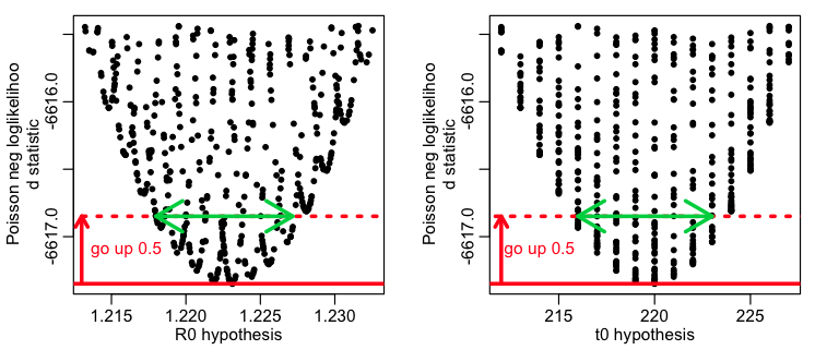
This method has the advantage that it is easy to understand how to execute (once you’ve seen a few examples). However, we talked about the fact that this procedure is only reliable if you have many, many sweeps of the model parameter values (for instance, the above plots are pretty sparsely populated, and it would be a bad idea to trust the confidence intervals seen in them…. they are underestimated because the green arrows don’t quite reach to the edge of the parabolic envelope that encases the points).
The fmin+1/2 method also does not yield a convenient way to determine the covariance between the parameter estimates, without going through the complicated numerical gymnastics of estimating what is known as the Hessian matrix. The Hessian matrix (when maximizing a log likelihood) is a numerical approximation of the matrix of second partial derivatives of the likelihood function, evaluated at the point of the maximum likelihood estimates. Thus, it’s a measure of the steepness of the drop in the likelihood surface as you move away from the best-fit estimate.
It turns out that there is an easy, elegant way, when using the graphical Monte Carlo method, to use information coming from every single point that you sample to obtain (usually) more robust and reliable parameter estimates, and (usually) more reliable confidence intervals for the parameters.
The weighted means method
To begin to understand how this might work, first recall from the previous module that the fmin+1/2 method gives you the one standard deviation confidence interval. Recall that to get the S standard deviation confidence interval, you need to go up 0.5*S^2 from the value of fmin, and examine the range of points under that line. This means that when we plot our negative log likelihood, f, vs our parameter hypotheses, the points that lie some value X above fmin are, in effect sqrt(2*X) standard deviations away from the best-fit value. Here is what that looks like graphically:
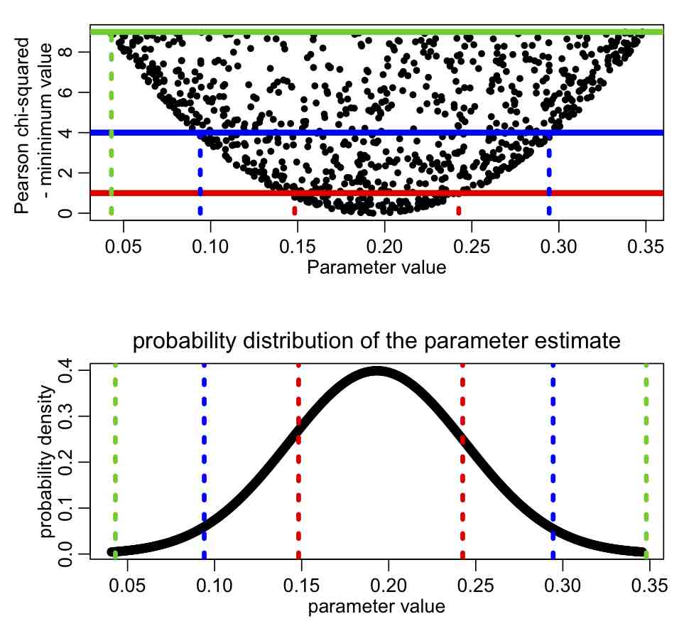
The red lines correspond to the points that lie at fmin+1/2 (the one standard deviation confidence interval), the blue lines correspond to the points that lie at fmin+0.5*2^2=fmin+2 (the two standard deviation confidence interval), and the green lines correspond to the points that lie at fmin+0.5*3^2=fmin+4.5 (the three standard deviation confidence interval).
It should make sense to you that the points that are further away from fmin carry less information about the best-fit value compared to points that are have a negative log likelihood close to the minimum. After all, when using the graphical Monte Carlo method, you aim to populate the graphs well enough to get a good idea of the width of the parabolic envelope in the vicinity of the best fit value.
So… this suggests that if we were to take some kind of weighted average of our parameter hypotheses, giving more weight to values near the minimum in our negative log likelihood, we should be able to estimate the approximate best-fit value. Weighted averages are an average where some points are given greater importance, or ‘weight’, in the calculation of the average. It is similar to an ordinary arithmetic mean (the most common type of average), except that instead of each of the data points contributing equally to the final average, some data points contribute more than others.
It turns out that the weight that achieves this in our graphical Monte Carlo procedure is intimately related to those confidence intervals we see above. If we do many Monte Carlo iterations of the parameter sampling procedure, sampling our parameter hypotheses and calculating the corresponding negative log likelihoods, f, we can estimate our best fit values by taking the weighted average of our parameter hypotheses, weighted with weights
w=dnorm(sqrt(2*(f-fmin)))
where dnorm is the PDF of the Normal distribution. Don’t worry yourself too much about how that expression was derived… there is a whole lot of statistical theory behind it, that you don’t need to necessarily understand in order to apply it.
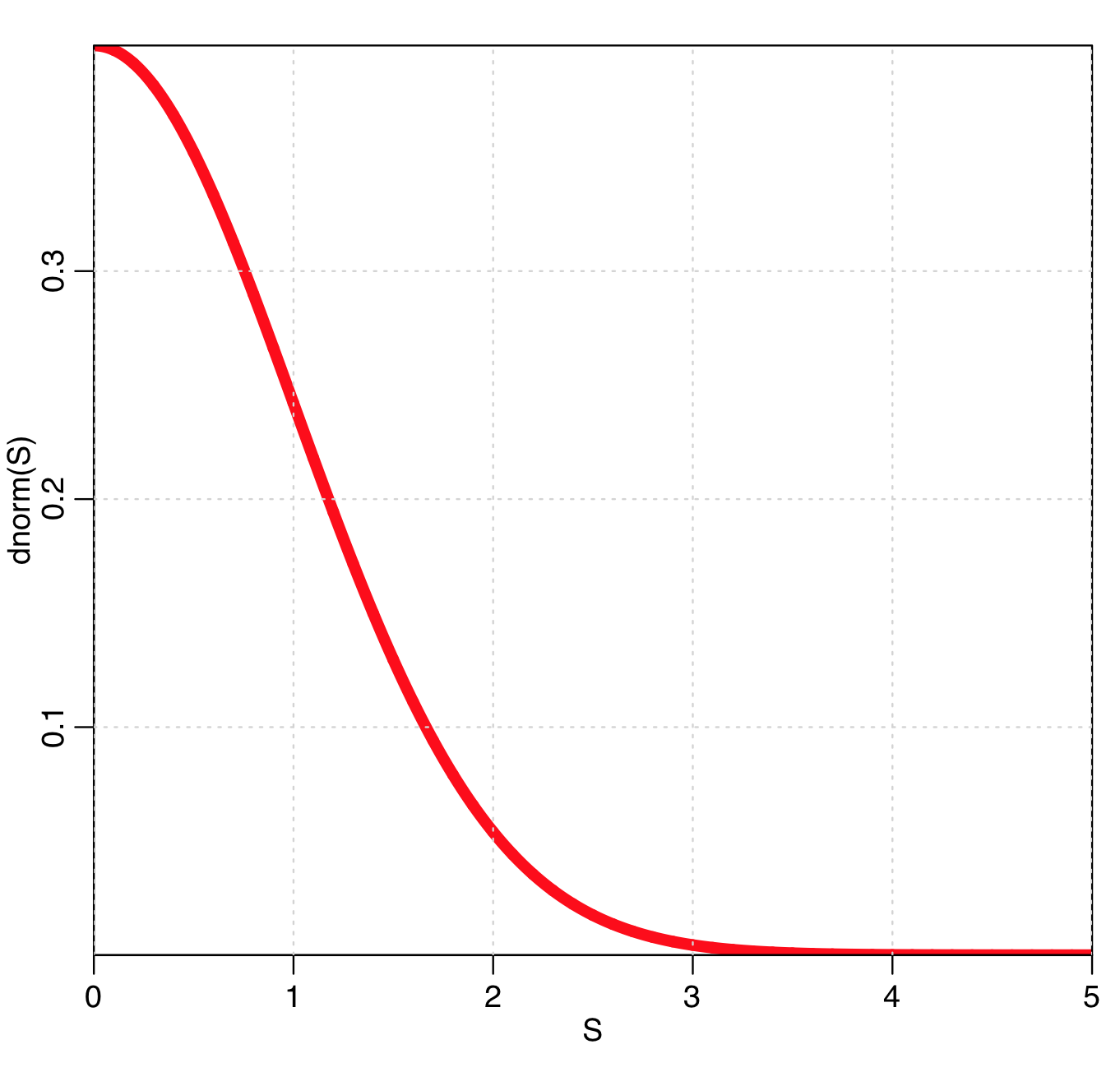
Notice that w is maximal when f=fmin, and gets smaller and smaller as f moves away from fmin. In fact, when f=fmin+0.5*S^2 (the value that corresponds to the S std dev CI), then
w=dnorm(S)
So, the points that are close to giving the minimum likelihood are given a greater weight in the fit, because they are more informative as to where the minimum actually lies. The plot of w vs S is:
Thus, the further f gets away from fmin, the less weight the points are given, but they still have some weight. This means that every single set of parameter hypotheses you sample in the graphical Monte Carlo procedure can give some information as to the best-fit average values of the parameters… this is very nice, because just using the fmin+1/2 method requires many, many iterations of the Monte Carlo procedure in order to obtain densely populated plot to achieve this.
Estimating the best-fit, and variance (one-standard deviation) and co-variance of parameter estimates using the weighted means method
It turns out that not only can these weights be used to estimate our best-fit values, they also can be used to estimate the covariance matrix of our parameter estimates. If we have two parameters (for example), and we’ve randomly sampled N_MC parameter hypotheses, we would form a N_MCx2 matrix of these sampled values, and then take the weighted covariance of that matrix. The R cov.wt() function does this. Here’s an example of what this might look like, if we were (for example) fitting a model with two parameters, R0 and t0:
       weight = dnorm(sqrt(2*(vneglog_likelihood-min(vneglog_likelihood))))

       R0_best_weight = weighted.mean(vR0,weight)
       t0_best_weight = weighted.mean(vt0,weight)

       A = cov.wt(as.matrix(cbind(vR0,vt0,valpha)),weight,cor=T)
       Vcov_weight_method = A$cov
       eR0_best_weight = sqrt(Vcov_weight_method[1,1])
       et0_best_weight = sqrt(Vcov_weight_method[2,2])
Advantages and disadvantages of the weighted mean method
Advantages of the weighted mean method: with this method every single point you sample gives information about the best-fit parameters and the covariance matrix for those parameter estimates. Unlike the fmin+1/2 method, where it is only those points right near the minimum value of f and at fmin+1/2 that really matter in calculating the confidence interval.
Also, using this weighted method you trivially get the estimate covariance matrix for the parameters, unlike the fmin+1/2 method where this would be much harder to achieve. The variance estimate for each of the parameters is the diagonal of this matrix, and the one-standard deviation estimates are the square roots of the diagonal elements (recall that the variance is the one-standard deviation squared).
Another advantage of the weighted means method is that you don’t have to populate your plots quite as densely as you would for the fmin+1/2 method in order for it to reliably work; this is because every single point you sample is now informing the calculation of the weighted mean and weighted covariance matrix.
The disadvantage of this method is that you must uniformly randomly sample the parameters (no preferential sampling of parameters using rnorm for instance), and you must uniformly sample them over a broad enough range that it encompasses at least a three or four standard deviation confidence interval; otherwise, as we’ll see, you will underestimate the parameter uncertainties).
Also, the weighted mean method should not be used in fits where the parabolic envelopes when plotting the negative log-likelihood vs parameter hypotheses are highly asymmetric in the vicinity of the best-fit value. This is because the weighted mean method inherently assumes that envelope is symmetric. Do not use the weighted means method when the envelopes are high asymmetric!
An example: fit of SIR model to influenza data
As an example of how this works, let’s return to the seasonal influenza SIR model we have used as an example in several other modules. Our data was influenza incidence data from a seasonal influenza epidemic in the midwest in 2007-08, and we fit the transmission rate, beta (or alternatively, R0=beta/gamma), of an SIR model to this data.
The R script fit_midwest_negbinom_gamma_fixed.R fits to this data using both the fmin+1/2 method and the weighted means method. The script reads in the data midwest_influenza_2007_to_2008.dat . You will also need the file sir_func.R that has the function that calculates the derivatives for the SIR model.
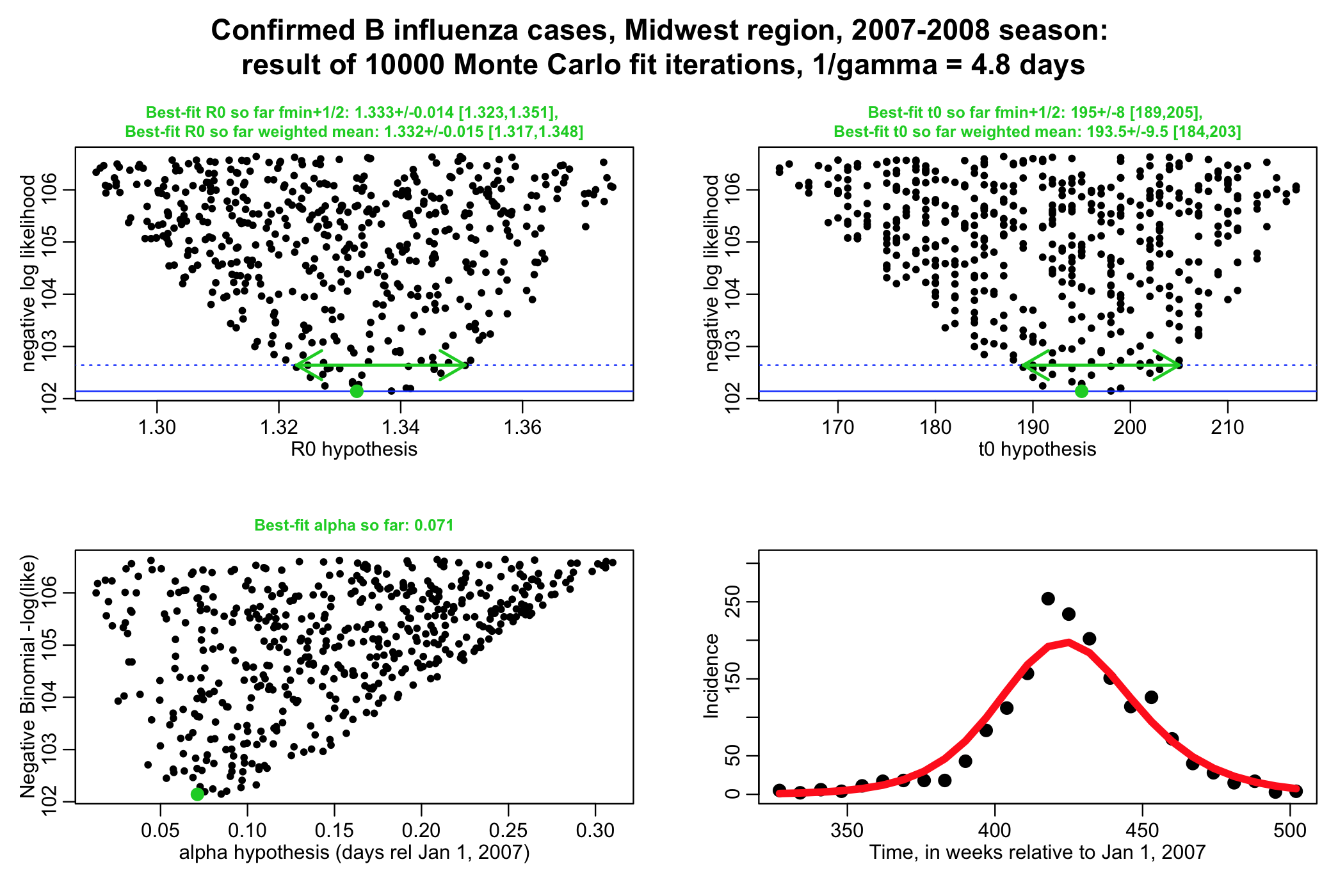
The script performs a negative binomial likelihood fit to the influenza data, assuming that the average recovery period, 1/gamma, for flu is fixed at 4.8 days. The script produces the following plot (recall that alpha is the over-dispersion parameter for the negative binomial likelihood, and t0 is the time of introduction of the virus to the population.
The script gives the best-fit estimate using the graphical Monte Carlo fmin+1/2 method, and also the weighted mean method. Note that the plots should be much better populated in order to really get trustworthy estimates from the fmin+1/2 method:
To see how the parameter values covary, after the script has finished running, type
A = cov.wt(as.matrix(cbind(vR0,vt0,valpha)),weight,cor=T)
A$cor
This yields:
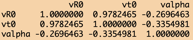
We can see that the parameters R0 and t0 are highly correlated (ie: as t0 goes up, R0 has to also adjust upwards to fit to the data, and vice-versa). This makes sense: the higher the R0, the earlier an outbreak peaks after it begins.
In order to get the covariance matrix without using the weighted mean method, we would have to numerically estimate the Hessian matrix for our SIR model negative log likelihood in the vicinity of the best-fit value:
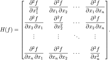
where f is our negative log-likelihood and the x are the parameters. Especially when using the Negative Binomial fit, this amounts to the mother-of-all partial derivative calculations, and each of those partial derivatives has to be solved numerically, because our model can only be solved numerically.
It is so much easier to use the weighted mean method!
Another example, this time with simulated data: compare weighted mean covariance estimate to that from Hessian
As another example of how this works in practice, let’s return to the simple example we saw in this previous module, where we compared the performance of the fmin+1/2 method to that where we analytically calculate the Hessian to estimate the parameter uncertainties.
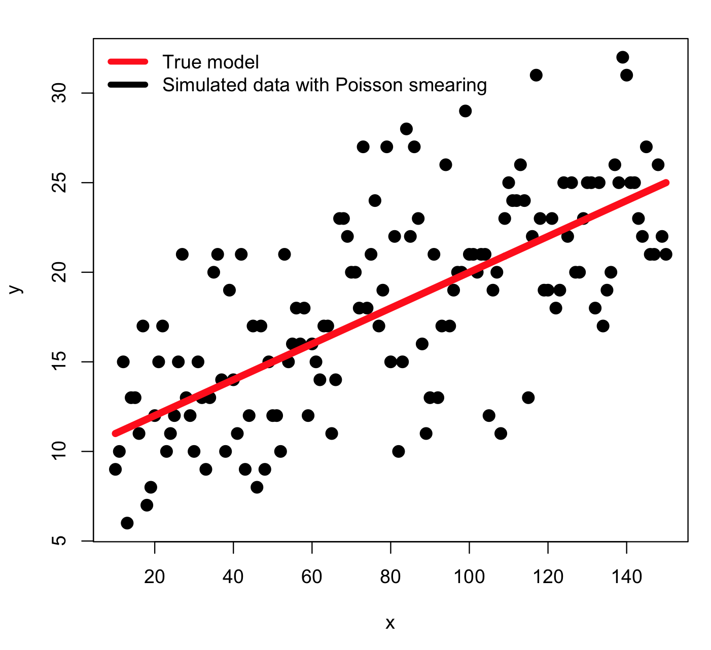
In the example, the model we considered was y=a*x+b, where a=0.1 and b=10, and x goes from 10 to 150, in integer increments. We simulate the stochasticity in the data by smearing with numbers drawn from the Poisson distribution with mean equal to the model prediction. Thus, an example of the simulated data look like this:
Recall that the Poisson negative log likelihood looks like this
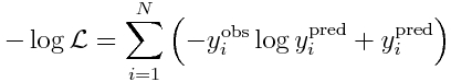
where the y_i^obs are our data observations, and y_i^pred are our model prediction (y_i^pred = a*x_i+b).
In the example hess.R, we randomly generated many different samples of our y^obs, and then used the Monte Carlo parameter sweep method to find the values of a and b that minimize the negative log likelihood. Then we calculated the Hessian about this minimum and estimated the one-standard deviation uncertainties on a and b from the covariance matrix that is the inverse of the Hessian matrix. Recall that the square root of the diagonal elements of the covariance matrix are the parameter uncertainties.
We also did this using the fmin plus a half method, to show that If the fmin plus a half method works, its estimate of the one-standard-deviation confidence intervals should be very close to the Hessian estimate.
We can add into this exercise our weighted mean method. The R script hess_with_weighted_covariance_calculation.R does just this.
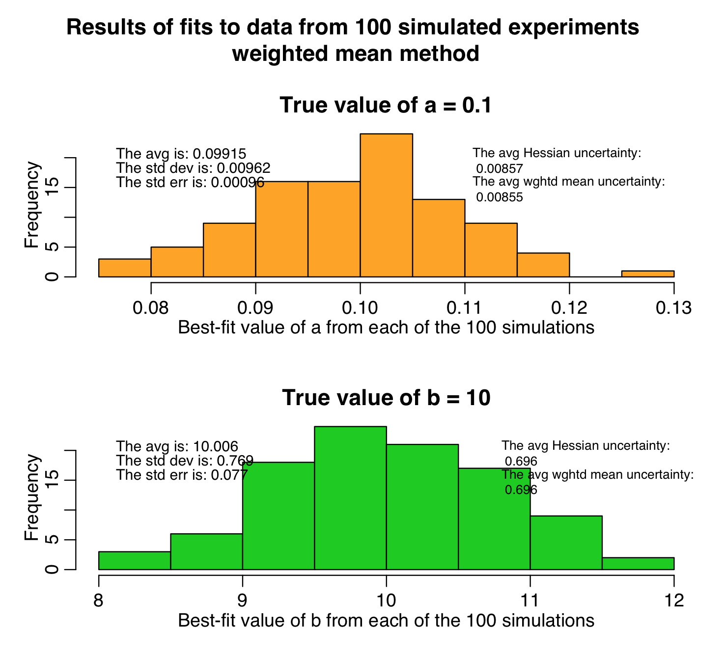
The script produces the following plot, histogramming the parameter estimates from the weighted mean method. As you can see, the estimates are unbiased, and the uncertainties on the parameters assessed by the weighted mean method are very close to those assessed by the analytic Hessian method:
The script also produces the following plot:
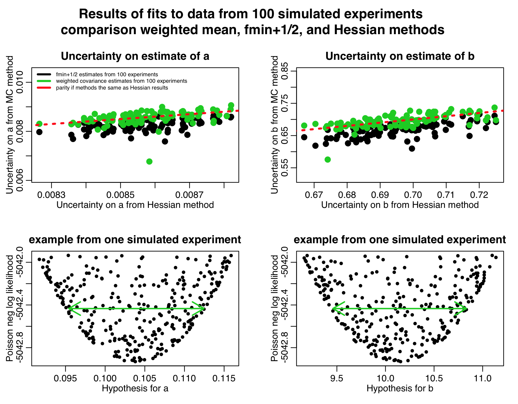
Notice in the top two plots that the parameter uncertainties assessed by the weighted mean method are quite close to those estimated by the Hessian method, but the uncertainties assessed by the fmin+1/2 method are always underestimates. This is because we didn’t sample that many points in our graphical Monte Carlo procedure, as can be seen in the examples in the two bottom plots; the plots are so sparsely populated, the green arrows that represent the CI’s estimated by the fmin+1/2 method don’t go all the way to the edge of the parabolic envelope.
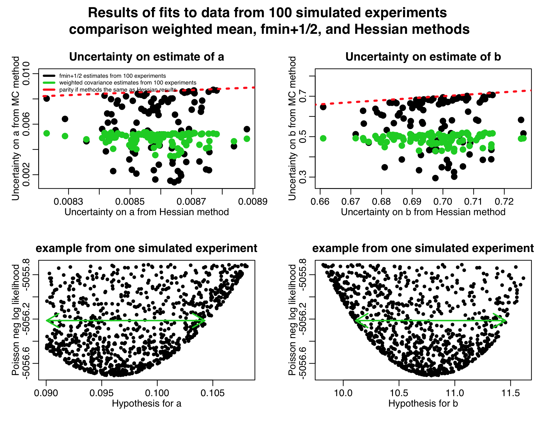
So, even with relatively sparsely populated plots, the weighted mean method works quite well. If they are really, really sparsely populated, however, you will find that the performance of the method starts to degrade; take a look at what happens when you change nmc_iterations from 10000 in to 100 in hess_with_weighted_covariance_calculation.R:

The estimates of the parameter uncertainties still are scattered about the Hessian estimates (and the fmin+1/2 method miserably fails due to the sparsity of points). However, notice that there is quite a bit of variation in the uncertainty estimates using the weighted mean method about the red dotted line (compare to the other plot, above); the more MC iterations you have, the more closely these will cluster about the expected values (ie; the more trustworthy your parameter uncertainty estimates will be). So, don’t skimp on the MC parameter sampling iterations, even when using the weighted mean method! In general, with this method, you need to run enough MC parameter sweep iterations to get a reasonable idea of the parabolic envelope in the vicinity of the best-fit value.
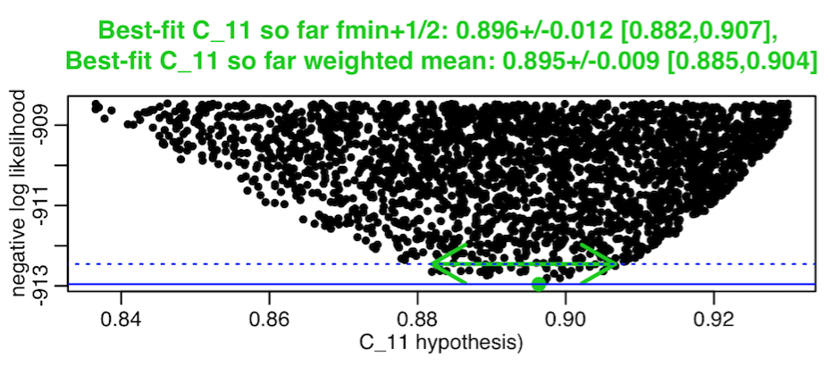
One catch of this method, as mentioned above, is to ensure that you do your random uniform parameter sweeps over a broad enough area… if you sample parameters to close to the best-fit value, the weighted mean method will underestimate the confidence intervals. In general, you have to sweep at least a four standard CI. As an example of what occurs when you use too narrow a range, instead of sampling parameter a uniformly from 0.06 to 0.14, uniformly sample it from 0.09 to 0.11 in the original hess_with_weighted_covariance_calculation.R script. We now get:
You can see that the confidence intervals are now severely under-estimated by the weighted mean method.
It needs to be kept in mind that the covariance matrix returned by the weighted mean method assumes that the confidence interval is symmetrically distributed about the best-fit value. In practice, this isn’t always the case; sometimes the plots of the neg log likelihood vs parameter hypotheses, instead of looking like they have a symmetric parabolic envelope, have a highly asymmetric parabolic envelope, like this, for example:
The weighted mean method will essentially produce a one standard deviation estimate that is derived from an “average” symmetric parabola fit to the asymmetric parabola. It will tend to underestimate confidence intervals in such cases. When you have highly asymmetric parabolic envelopes in your plots of the neg log likelihood vs your parameter hypotheses, it is thus best to use the fmin+1/2 method.