For our models, we often obtain estimates of some of the parameters from prior studies in the literature.  For example, for most diseases, the incubation and infectious periods are usually estimated from observational studies.  For animal populations, the birth rates are also usually estimated from observational studies. 

However, these parameter estimates in the literature are not a fixed exact value, and have uncertainties associated with them.  Those uncertainties, when properly taken into account in our fits using the graphical Monte Carlo method, will feed into the uncertainties on the parameters we are trying to fit for. In this module, we will discuss how to incorporate this “prior-belief” of known parameters and their uncertainties into our graphical Monte Carlo fits.

Incorporating parameter prior-information into the fit

For many models, information about the parameters and/or initial conditions can be obtained from other studies. For instance, let’s examine the seasonal influenza SIR model we have used as an example in several other modules.  Our data was influenza incidence data from an influenza epidemic in the midwest, and we fit the transmission rate, beta (or alternative, R0=beta/gamma), of an SIR model to this data. For example, using the R script fit_midwest_negbinom_gamma_fixed.R

The script performs a negative binomial likelihood fit to the influenza data, assuming that the average recovery period, 1/gamma, for flu is fixed at 4.8 days.  The script produces the following plot (recall that alpha is the over-dispersion parameter for the negative binomial likelihood, and t0 is the time of introduction of the virus to the population.

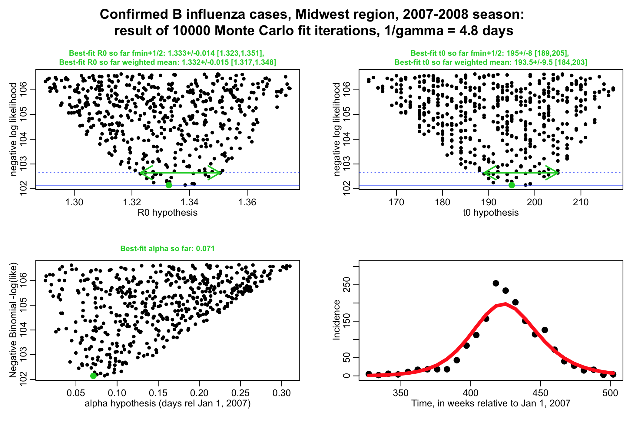
The script gives the best-fit estimate using the graphical Monte Carlo fmin+1/2 method, and also the weighted mean method.  Note that the plots should be much better populated in order to really get trustworthy estimates from the fmin+1/2 method.

In reality, most of our parameters that we obtain from prior studies aren’t know to perfect precision

In our script above, we assumed that 1/gamma was 4.8 days based on a prior study in the literature. However, this was estimated from observational studies of sick people, and, in reality, there are statistical uncertainties associated with that estimate.  In the paper describing the studies, they state that their central estimate and 95% confidence interval on 1/gamma was 4.80 [4.31,5.29] days.  Unless told otherwise in the paper from which you get an estimate, you assume that the uncertainty on the parameter is Normally distributed.  Because the 95% CI is +/-1.96*sigma from the mean, this implies that the std deviation width of the Normal distribution is sigma=(4.8-4.31)/1.96~0.25 days

Thus, our probability distribution for x=1/gamma is

P(x|mu,sigma)~exp(-0.5(x-mu)^2/sigma^2)

with mu=4.8 days, and sigma = 0.25 days, in this case.

 

Uncertainty on “known” parameters affects the uncertainties on the other model parameters you estimate from your fit to data!

The uncertainty on 1/gamma will affect the uncertainty on our parameter estimates.  For instance, is it clear that if all we know about 1/gamma was that it was between 1 and 10 days, it would be much harder to pin down our transmission rate? (ie; we had no idea what 1/gamma was, and thus had fit for gamma, as well as R0, t0, and alpha)  The script fit_midwest_negbinom_gamma_unconstrained.R does this, and produces the following plot:

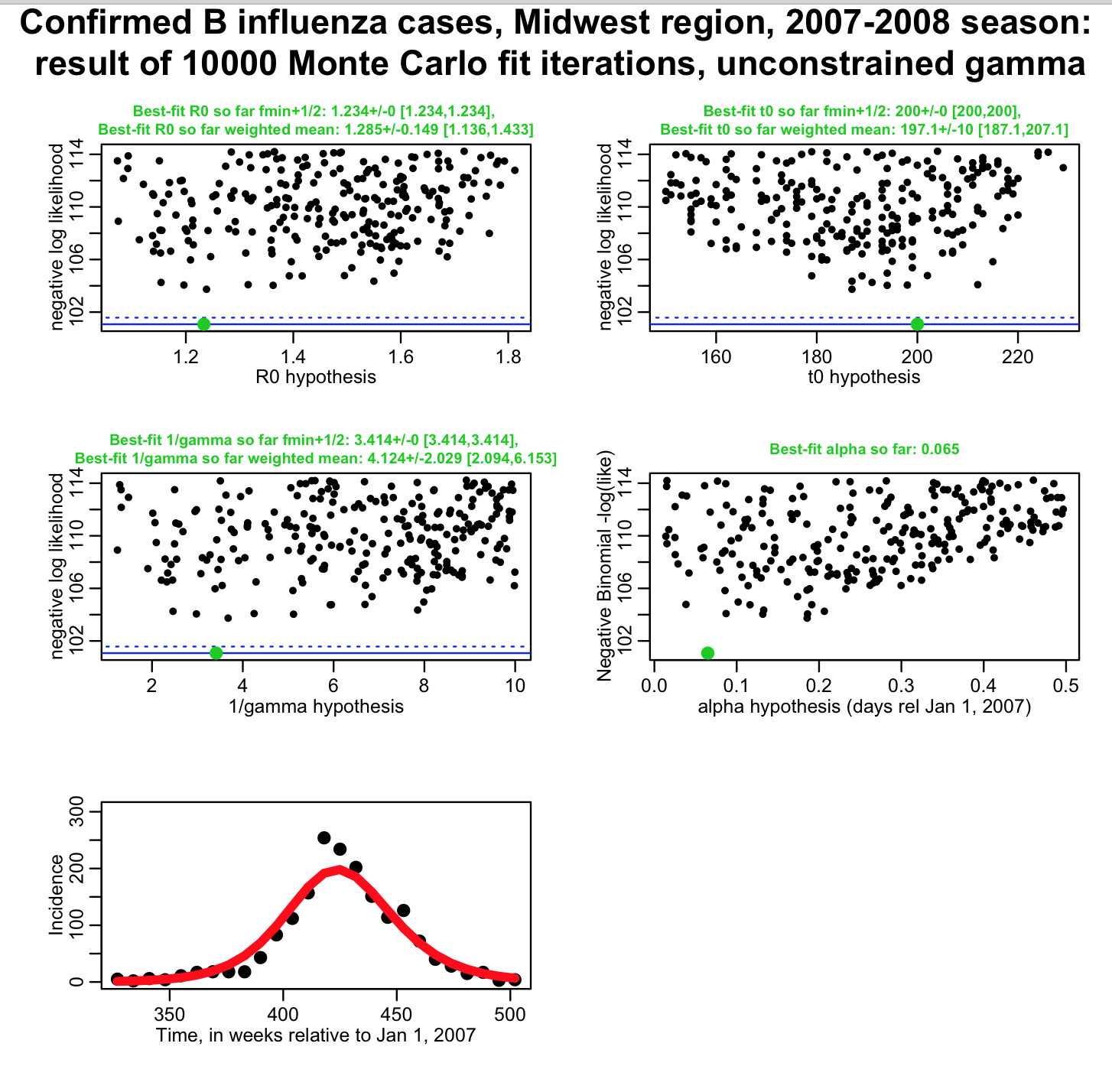
You can see that the influenza data we have perhaps give us a little bit of sensitivity to the parameter gamma, but not much (basically, the fit just tells us 1/gamma is somewhere between 2 to 6 days, with 95% confidence).  The uncertainties on our estimates of R0 and t0 have gone way up, compared to the first fit where we assumed 1/gamma was fixed at 4.8 days!  Also, when you are using the weighted mean method to estimate parameters and the parameter uncertainties, you can also get the covariance matrix for your parameter estimates.  The correlation matrix, derived from the covariance matrix, for this fit looks like this:

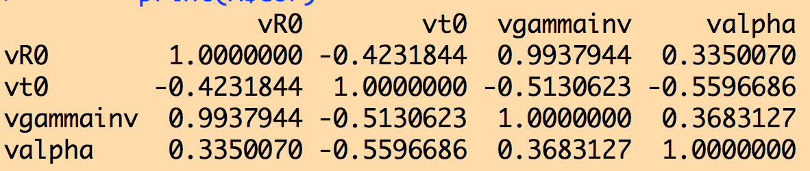
Notice that our estimates of R0 and 1/gamma are almost 100% correlated (this means that as 1/gamma goes up, R0 also has to go up to achieve a good fit to the data).    This is known as “covariance” of the parameters.

You never want to see parameters so highly correlated in your fits… it means that your best-fit parameters likely won’t give you a model with good predictive power for a different, equivalent data set (say, influenza data for the same region for the next flu season).

So, even though we seem to have a little bit of sensitivity to the value of 1/gamma in our fit, having that estimate 100% correlated to our estimate of R0 is not good, and a sign you shouldn’t trust the results of the fit.  It is better that we get values of gamma from the literature (which we should be doing anyway, because the recovery period can be directly estimated simply by observing patients).

Incorporating uncertainties on “known” parameters from the literature in our fit likelihoods

In order to take into account the uncertainties on our “known” parameter, x, you simply modify your fit likelihood to include the likelihood coming from the probability distribution for that parameter.  Thus, the negative log likelihood is modified like so:

negloglike = negloglike + 0.5*(x-mu)^2/sigma^2

Then, in the fit, you do Monte Carlo sampling not only of all your other unknown parameters (like R0, t0, and alpha in this case), but also uniformly randomly sample parameter x over a range of around approximately mu-4*sigma to mu+4*sigma.

For 1/gamma, we know that mu=4.8 days, and sigma is 0.25 days.  The R script fit_midwest_negbinom_gamma_constrained.R modifies the likelihood to take into account our probability distribution for our prior estimate of 1/gamma from the literature.  The script produces the following plot:

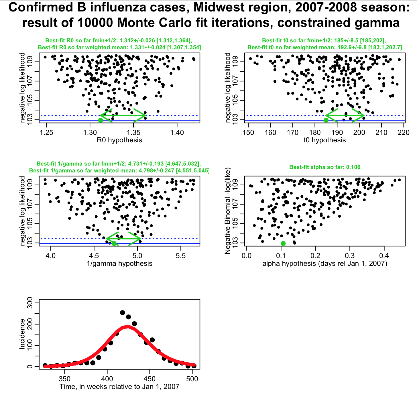
(again, for the fmin+1/2 method, we’d like to see these plots much better populated!).  Note that now our uncertainties on R0 and t0 from the weighted mean method are much smaller than they were when 1/gamma was completely unconstrained, but larger than they were when 1/gamma was fixed to 4.8 days.  By modifying the likelihood to take into account the probability distribution of our prior belief for 1/gamma, we now have a fit that properly feeds that uncertainty into our uncertainty on R0 and t0.

When publishing analyses that involve fits like these, it is important to take into account your prior belief probability distributions for the parameter estimates you take from the literature.  In some cases, your fit might be quite sensitive to the assumed values of those parameters; if the literature estimates are a bit off from what your data would “like” them to be to obtain a good fit, and you just assume a fixed central value for the parameter, sometimes you just won’t be able to get a good fit to your data.

When you include the parameter in your fit with a modified likelihood to take into account its prior belief probability distribution, the estimate you get from the fit to your data is known as the “posterior” estimate.  Note that the posterior estimate, and uncertainty, on 1/gamma that we obtained from fit_midwest_negbinom_gamma_constrained.R  is 4.798+/-0.247, and is pretty darn close to our prior belief estimate of 4.8+/-0.25.  If our data were sensitive to the value of 1/gamma, our posterior estimate would have a smaller uncertainty than the prior belief estimate, and likely have a different central value too.  In this case, they are almost identical, meaning that our data do not provide much sensitivity to this parameter.

Step-by-step guide

1. Identify parameters in your models for which there are pre-existing estimates in the literature
2. Write the code to do your fits with the graphical Monte Carlo method, assuming that the “known” parameter values are held fixed to the values from the literature, and only randomly sampling the other values.
3. Now, from the information in the literature, determine the average value of the parameter estimates, and one standard deviation uncertainty.  If all the literature provided was a range, assume that is the 95% CI.  The average value estimate is thus mu=0.5*(upper_range+lower_range), and the estimate of sigma is thus sigma=0.5*(upper_range-lower_range)/1.96
4. Modify the negative log likelihood in your fit with the following term:  negloglike = negloglike + 0.5*(x-mu)^2/sigma^2
5. Redo your graphical Monte Carlo procedure, now also randomly sampling your “known” parameter in the range mu-4*sigma to mu+4*sigma.
6. Use the fmin+1/2 method to obtain the best-fit parameter estimates and their uncertainties.
7. You will find the uncertainties on your “unknown” parameters will now be larger than what they were when you had simply held the “known” parameters fixed in the fit.  This is because those uncertainties not properly incorporate the uncertainties on your “known” parameters.
8. If your data turn out to be sensitive to your “known” parameter, you may have to adjust the range over which you sample that parameter if you notice the minimum value of the negative log likelihood is right at the edge of your mu-4*sigma,mu+4*sigma sampling range.  If that occurs, adjust the ranges and re-do the fits.  The fact that your data provide sensitivity to that parameter, and your posterior parameter estimate is different than what is seen in the literature is an interesting addition to the Discussion section of your paper!

If you have “known” parameter estimates from the multiple sources in the literature, and those estimates don’t agree, as a robustness cross-check do your fits with each of the parameter estimates in turn.  The optimal choice among those estimates is the one that returns the lowest best-fit negative log-likelihood to your data.  This is an interesting addition to the Discussion section of your paper!

Also, note that if you use uniform random sampling of your parameters for all parameters (including the parameter you want to constrain), you can easily apply the additional constraint on the negative log likelihood after you have done all your Monte Carlo iterations.
Simply add in the constraint to the negative log likelihood, and make your plots of the new modified negative log likelihood versus the parameter hypotheses.  As long as your best-fit value for your constrained parameter is not bumped up agains the upper or lower edge of the sampling range, you’re fine.  This is what is known as a “post-hoc” constraint, because you apply it after you’ve done all your Monte Carlo iterations.  If it is bumped up against the edge of the range, unfortunately you will have to repeat the Monte Carlo sampling procedure again, with broader ranges for that parameter.