[After reading through this module, students should have an understanding of contact dynamics in a population with age structure (eg; kids and adults). You should understand how population age structure can affect the spread of infectious disease. You should be able to write down the differential equations of a simple SIR disease model with age structure, and you will learn in this module how to solve those differential equations in R to obtain the model estimate of the epidemic curve]

Contents:

• Introduction
• Population contact patterns
• An example of a contact matrix: kids and adults
• SIR model with age structure
• The reproduction number of the age structured SIR model
• R code for simulating an age structured SIR model
• Other kinds of class structure
• Things to try

Introduction

In a previous module I discussed epidemic modelling with a simple Susceptible, Infected, Recovered (SIR) compartmental model.  The model presented had only a single age class (ie; it was homogenous with respect to age).  But in reality, when we consider disease transmission, age likely does matter because kids usually make more contacts during the day than adults. The differences in contact patterns between age groups can have quite a profound impact on the model estimate of the epidemic curve, and also have implications for development of optimal disease intervention strategies (like age-targeted vaccination, social distancing, or closing schools).

Population contact patterns

Quantifying what entails a “contact” that is sufficient to transmit a disease can be extraordinarily difficult, especially with a disease like influenza that can be spread with even casual incidental contact with an infected person.  For influenza, social survey information is often used to quantify contacts, with probably one of the most comprehensive of these being the Mossong et al survey; they asked 7300 people of many different ages in 8 European countries to record the location (ie; work, home, school, etc), duration, and nature (ie; was touching involved) of all contacts they made during the day.  The participants also recorded the age of their contacts.

This incredibly rich data source can be transformed into what is known as a contact matrix (that is to say, the number of contacts per day a person of age i makes with a person of age j).  These contact matrices can look very pretty, especially if you make high contact rates warm colors, and low contact rates cold colors:

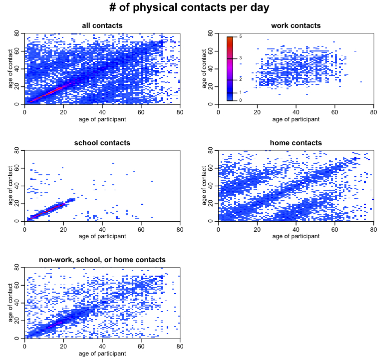
Notice that there is a strong tendency for people to prefer contacts with their peers.  Can you also see that children also have a preference for contacting people around 20 to 25 years older than they are (particularly in contacts that occur at home)?  And that adults have a preference for contacting people 20 to 25 years younger than they are (again, especially in home contacts)?  This is due to child/parent and parent/child interactions.  In the contact matrix for home contacts you can even see evidence of grandchild/grandparent and grandparent/grandchild interactions.

An example of a contact matrix: kids and adults

Let’s assume we have a population with two age classes; kids and adults.  Kids are f_1=25% of the population, and adults are the rest.  Further, let’s assume that kids make 27 contacts each day, 2/3 of which are with other kids.  Assume that adults make 15 contacts each day.  The contact matrix is

How did I know that C_21 was going to be 3?  Because the matrix has to satisfy reciprocity, meaning that within the population the total time spent by kids with adults has to equal the total time spent by adults with kids.  Thus we must have f_i*C_ij = f_j*C_ji  All contact matrices have to satisfy this condition.  Note that in our contact matrix we are considering all contacts, not just the kind of contacts that might transmit infection.  When we use this contact matrix in disease modelling, we will scale it to reflect “probability of transmission on contact”.

SIR model with age structure

The system of ordinary differential equations for a SIR model with age structure includes the contact matrix, and looks like this:

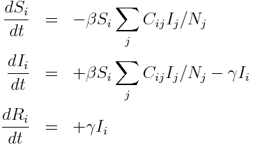
where i and j are the indices of the age classes, and N_j is the population in age group j.  The quantity beta is the probability of transmission on contact.  The quantity gamma is the recovery rate.  Note that in this simple model we assume that beta and gamma are the same for all age classes.  This might not be true, and is an example of how this model can be extended.  For now we will just consider the simplified case.

Note that this model doesn’t include deaths or births, immigration or emigration, and also assumes that the time-frame of the epidemic is so short that a significant number of people in age class i don’t end up in age class j by the end of the epidemic.

The reproduction number of the age structured SIR model

An excellent paper introducing how to calculate the reproduction number of compartmental models of disease transmission using the Next Generation Matrix method is P. van den Driessche (2016).

Mathematical analysis of the age structured SIR  model using this method reveals that the reproduction number is equal to beta/gamma times the largest eigenvalue of the matrix M, where M has elements M_ij = C_ij f_i/f_j

For our two age-class example, the R0 is thus (beta/gamma)*9.93.  Since we often have an estimate of the R0 of a disease like influenza from analysis of the rate of exponential rise of an epidemic (and we know the recovery rate, gamma, from observational studies of infected people), we can thus estimate the probability of transmission on contact.  For our hypothetical population with contact patterns described by C above, and a pandemic-like influenza strain with R0=1.5, and 1/gamma=3 days, we can thus estimate that the probability of transmission on contact with an infected person is around 0.05.

Note that the probability of transmission on contact folds in a bunch of different factors: for instance, it can be affected by the average proximity of contact, and also by the transmissibility of the flu strain itself (some strains of flu readily transmit between humans, but other strains, like H5N1, don’t).  Thus the R0 of a flu strain depends not only intrinsically on the transmissibility of the strain itself, but also on human behavioral patterns that may make transmission more probable if people are crowded, or shaking hands or kissing a lot.

R code for simulating an age structured SIR model

The file sir_age.R contains an R script to numerically solve the system of ODE’s above for an age-structured SIR model with two age classes. I assume that kids are 25% of the population, and that the contact matrix is the same that I gave above. I also assume that we are modelling a hypothetical pandemic influenza outbreak with R0=1.5, and that the recovery period is 1/gamma=3 days.  To run the script, download it, and make sure you have the odesolve package installed in R, and that the working directory in R is the same directory sir_age.R is in.  Then type

source("sir_age.R")

The following plot will be produced, showing the influenza prevalence in each of the age groups as the epidemic progresses:

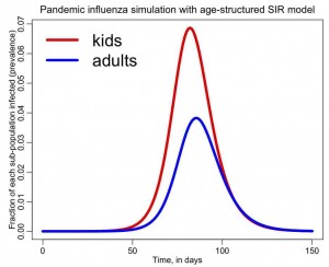
You can see that the prevalence is higher in kids, and this is because of their higher contact rates.  Children a super-spreaders of flu in the population, which is why it has been suggested that it is best to target vaccinations at that age group (even though most flu mortality is in the elderly).  It has also been noted that flu incidence in the elderly can be significantly reduced with even modest reduction of contact between grandchildren and grandparents during the flu season.

Other kinds of class structure

In this discussion we only looked at epidemic modelling with age structure.  However, the model in the Equations above could easily be generalized to instead represent other stratifications within the population that may impact the spread of disease. An example is the male/female population structure that needs to be taken into account when modelling the spread of diseases like AIDS.

Things to try

Keep the row sums of the C matrix the same, but make all the contacts peer-to-peer (ie; all non-diagonal elements in C are the same).  Given the probability of transmission on contact beta=0.05, how does this change the shape of the epidemic curve and final size estimate, relative to the previous estimates we obtained with the original sir_age.R file?

Examine the effect of reducing just the kid-to-kid interactions in the C matrix given above (assume that beta=0.05).  This is equivalent to closing schools.  How does the final size of the epidemic depend on the fractional reduction in kid-to-kid contacts?

How about vaccinations?  If you only have enough vaccines to vaccinate 20% of the population, how should those be apportioned between kids and adults to optimize the reduction in the overall epidemic final size.