
[In this module, students will learn about probability distributions important to statistical modelling, focussing primarily on probability distributions that underlie the stochasticity in time series data.
In addition, in this course we will be learning how to formulate figure-of-merit statistics that can help to answer research questions like “Is quantity A significantly greater/less than quantity B?”, or “Does quantity X appear to be significantly related to quantity Y?”. As we are about to discuss, statistics that can be used to answer these types of questions do so using the underlying probability distribution to the statistic. Every statistic used for hypothesis testing has an underlying probability distribution.]
- Introduction
- Mean, variance and standard deviation of data
- Pearson’s correlation coefficient statistic
- Mean, variance and standard deviation of probability distributions
- Uniform probability distribution
- Exponential probability distirbution
- Normal probability distribution
- Introduction
- Hypothesis testing with Normally distributed data
- Other distributions approach the Normal distribution
- Functions in R related to the Normal distribution
- Sum and difference of two Normal distributions is also Normal
- Checking to determine if data are consistent with being Normally distributed
- Central Limit Theorem (CTL)
- CTL application: test if mean of sample is consistent with some value
- CTL application: are the means of two samples consistent with being the same
- CTL applications: Examples
- CTL applications: Things to ponder
- Students-t distribution
- Introduction
- Probability density function
- R functions related to Students-t distribution
- Comparing Students-t to Normal distribution
- The Students-t statistic
- Using the Students-t statistic to test if mean of a sample is consistent with some value
- Using the Students-t statistic to test if means of two samples are consistent with being equal
- Limits of using Students-t statistic for hypothesis testing of means.
- Using Students-t statistic to test significance of correlation coefficients
- Chi-square distribution
- Introduction
- Probability density
- R functions related to the chi-square distribution
- Using chi-square distribution to test if means of multiple samples are consistent with being the same
- Using Pearson chi-square test to determine if frequency of events is consistent with predicted
- Cautions when using Pearson chi-square test.
- Poisson distribution
- Negative binomial distribution
- Binomial distribution
Introduction
An understanding of various probability distributions is also needed if one wants to fit parameters of a statistical model to data, because the data we encounter in sociology/economics/biology/epidemiology/etc pretty much always have underlying stochasticity (randomness)a, and that stochasticity feeds into uncertainties in the fitted statistical model parameters. It is important to understand what kind of probability distributions typically underlie the stochasticity in our data.
In probability theory, the probability density function is the function of a random variable that describes the probability that the random variable can assume a specific value (for a discrete probability distribution, the term probability mass function is used). I will often (rather sloppily) refer to probability density and mass functions as probability distributions.
Before we move on to talking about probability distributions, first a quick refresher on two of the most important statistics we will be dealing with throughout this course; the mean and variance.
Mean, variance and standard deviation of a sample of random numbers (ie; data)
Given a distribution of n random numbers, X_i, the estimated sample mean is

If we know the true mean, mu, we can calculate the population variance as

However, in reality, we don’t know the true mean to plug into the above expression, we can only estimate it from the data. We thus estimate the true variance using a quantity known as the sample variance

where bar(X) is the mean of the X_i. The sample standard deviation is a measure of the spread in X_i, and is equal to the square root of the sample variance. Notice that the sample variance is undefined when n<2.
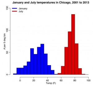
The R script chicago_weather.R reads in Chicago climate data between 2001 to mid-2003 that I downloaded from the Weather Underground website, and put into the file chicago_weather_summary.txt. It histograms the temperature data for all years for January and July, yielding the following plot (and also prints out the mean and sample variance calculated with the formulas above, and with R’s inbuilt functions mean() and var())
:
Correlation of paired data, (X_i,Y_i)
The Pearson correlation statistic (sometimes referred to as Pearson’s r) is a measure of the linear correlation (dependence) between two variables X and Y, giving a value between +1 and −1 inclusive, where 1 is total positive correlation, 0 is no correlation, and −1 is negative correlation. It is widely used in the sciences as a measure of the degree of linear dependence between two variables. If we have a sample of n pairs of data (X_i,Y_i) (say, for instance, X_i are the temperature on a series of days, and the Y_i are the humidity measurements on those same days), then the formula for the Pearson correlation coefficient statistic is
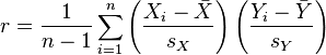
where s_x and s_y are the sample standard deviations.
The R function cor(x,y) calculates the Pearson correlation coefficient between a vector x and a vector y.
The R script chicago_pollution.R reads in the file chicago_pollution.txt that has daily pollution data for the city of Chicago from 2001 to 2012. The pollutants are ozone, SO2, NO2, CO, and fine particulate matter. The script also reads in climate data from the file chicago_weather_summary.txt. The script then plots the daily ozone reading vs the daily average temperature (which do you think would likely be the independent and dependent variables?), and calculates the Pearson correlation coefficient. We will discuss below how to determine if a correlation coefficient is statistically different than 0. The script produces the following plot: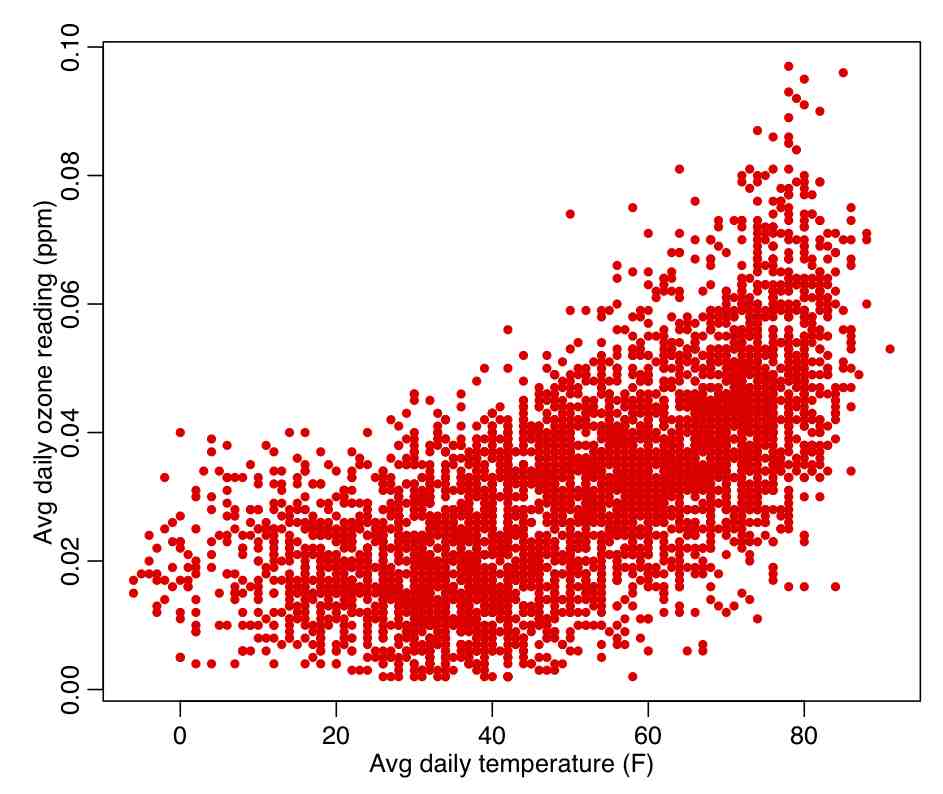
Mean, variance, and moments of probability distributions
If f(x) is the probability function for some distribution, then the moments of the distribution are defined as:
![<br /> \[<br /> {\rm zero'th~moment}~~M_0 =~\int_a^b ~f(x)~dx<br /> \]<br /> \[<br /> {\rm first~moment}~~M_1 =~\int_a^b ~x~f(x)~dx<br /> \]<br /> \[<br /> {\rm second~moment}~~M_2 =~\int_a^b ~x^2~f(x)~dx<br /> \]<br /> \[<br /> \vdots<br /> \]<br /> \[<br /> {\rm n'th~moment}~~M_n =~\int_a^b ~x^n~f(x)~dx<br /> \]<br />](http://www.ugrad.math.ubc.ca/coursedoc/math101/notes/moreApps/moments_3.gif)
The first moment is the mean, and the variance (a measure of spread) of the distribution is var=M_2-M_1^2.
Uniform probability distribution
One of the simplest probability distributions (conceptually at least) is the Uniform probability distribution with probability density:
![<br /><br /><br /><br /><br /> f(x)=\begin{cases}<br /><br /><br /><br /><br /> \frac{1}{b - a} & \mathrm{for}\ a \le x \le b, \\[8pt]<br /><br /><br /><br /><br /> 0 & \mathrm{for}\ x<a\ \mathrm{or}\ x>b<br /><br /><br /><br /><br /> \end{cases}<br /><br /><br /><br /><br />](http://upload.wikimedia.org/math/8/f/b/8fbfebfbb3dfa135da807a45374376d5.png)
- Thus, if a random variable is uniformly distributed between a and b, then the probability that it will assume any value between a and b is constant. Note that the probability distribution given above has the probability that its integral from x from negative to positive infinity is equal to 1 (ie; the probability that x is somewhere in that range has to be 1!). This property is true of all probability densities. The plot of this probability density looks like:

- Notice, as mentioned, that the graph shows all intervals of the same length on [a,b] are equally probable.
- It is easy to show that the mean and variance of the Uniform distribution are 0.5(a+b) and (b-a)^2/12, respectively.
- R has a function that generates random number from the uniform distribution called runif(n,a,b), where n is the number of random number you would like generated. If the optional arguments a and b are not provided, they default to 0 and 1. dunif(x,a,b) gives the probability density at point x, punif(x,a,b) gives the CDF at x, and qunif(p,a,b) returns the value of x that gives a CDF value of p.

Exponential probability distribution
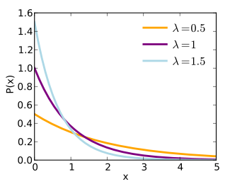
Another simple probability distribution is the Exponential distribution. It only has one parameter lambda, which is also known as the rate. The PDF is

The mean of the distribution is 1/lambda, and its variance is 1/lambda^2. The following shows the shape of the distribution for various values of lambda (note that the most probable value is always x=0, and that the distribution has long tails):
Normal Probability Distribution
The Normal (or Gaussian, or bell curve) distribution is also very commonly encountered in statistical model, and often (but certainly not always) underlies the stochasticity in data. It has the probability density function defined for all real x

Notice that the PDF is symmetric about mu. It is straightforward to show that the mean and variance of this distribution are mu and sigma^2, and it is also straightforward to show that it integrates to 1 over the range of x from minus to plus infinity. For various values of mu and sigma, the distribution looks like this:
It is common to indicate that a variable, for instance Z, is Normally distributed with mean mu and variance sigma^2 by writing

It is also important to note that if we transform Z by subtracting mu and dividing it by sigma, the resulting variable is distributed as N(0,1):

Hypothesis testing with Normally distributed data: How do we use a probability distribution like this for hypothesis testing? Well, assume we had a data point, X, that we hypothesize (based on our knowledge of the underlying process that generated the data, for instance) was drawn from the Normal distribution with mean 0 and sigma 1 (for example). This is known as a “null hypothesis”. If we have observed X=5, we can see that value lies in the extreme tails of the distribution, where the probability is very low indeed. However, if we observe X=1 we see there is a reasonable probability of that occurring. We want to have a hypothesis test that tests the probability that you would observe a value of X that high (or that low) just by mere random chance if the null hypothesis was true. That probability is called a “p-value”. To calculate the p-value, we would integrate the PDF from -inf to X (and also look at the integral of the PDF from x to +inf… these two integrals need to sum to 1, recall). If one of those values is small (say p<0.05) statisticians generally decide that there is significant evidence that the null hypothesis is false, and they reject the null. Note that here we are talking about hypothesis testing with the Normal distribution just as an example of a distribution that might be used in hypothesis testing; different statistics used for hypothesis testing have different underlying probability distributions, and if you hypothesize that the statistic X is drawn from a particular PDF and wish to test that hypothesis, you would just integrate the PDF from -inf to X, and see if the resulting p-value is either close to 1, or close to 0.
Note that a low p-value doesn’t mean that the null hypothesis was definitively wrong; it just means that it is unlikely.
Let’s get back to the Normal distribution….
Other distributions that approach Normal distribution: An interesting thing about the Normal distribution is that many other probability distributions approach the Normal distribution under certain conditions, and we will discuss this further as we discuss the various probability distributions later in this module.
Functions in R related to the Normal distribution: R has a function called rnorm(n,mean,sd) that generates n random number from the Normal distribution. If the optional arguments mean and sd (standard deviation) are not given, then they default to 0 and 1, respectively. The dnorm(x,mean,sd) and pnorm(x,mean,sd) functions return the PDF and CDF at x, respectively. It is the pnorm() function that is used to integrate the probability distribution between -inf to x in order to assess the p-value.
Sum and difference of two Normal distributions is also a Normal distribution: Another interesting thing about the Normal distribution is that the sum and difference of two Normally distributed random numbers is also Normally distributed. If X and Y are independent random variables that are normally distributed (and therefore also jointly so), then their sum is also normally distributed. i.e., if


and X and Y are independent, then
 Equation (1)
- If you want to subtract Y from X, then Z is also Normal with the form
 Equation (2)
Checking to determine if data are indeed consistent with being Normally distributed: Many of figure-of-merit statistics used for hypothesis testing have the underlying assumption that the data are sampled from some particular probability distribution (more often than not, the Normal distribution). Before applying such hypothesis tests, it is prudent to check that the data do indeed appear to be distributed according to the assumed underlying probability distribution. But how can we test to determine if our data are Normally distributed (for instance, is the Chicago temperature data above Normally distributed)?
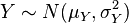
One means to do this is called a QQ-plot (the Q stands for “quantile“). The QQ-plot is an exploratory graphical device used to check the validity of a distributional assumption for a data set; the basic idea is to compute the theoretically expected value for each data point based on the distribution in question, based on the mean and standard deviation of the data. If the data indeed follow the assumed distribution, then the points on the QQ-plot will fall approximately on a straight line.
The R script fall_course_libs.R contains a function I wrote called norm_overlay_and_qq() that overlays a Normal distribution (with the same mean and standard deviation of the data) over a histogram of the data. If the data are Normally distributed, the pattern of histogram bins being higher/lower than the overlaid Normal curve should be more or less randomly up and down. A series of histogram bins that are too high are too low imply departure from Normality. The function also plots the QQ-plot of the data, comparing it to a Normal distribution, using the R qqnorm() function. The R script qqplot_examples.R creates three simulated data sets; the first is randomly sampled from the Normal distribution, the second is generated to be too peaked in the center compared to a Normal, and the third is generated to be skewed. It produces the following plot: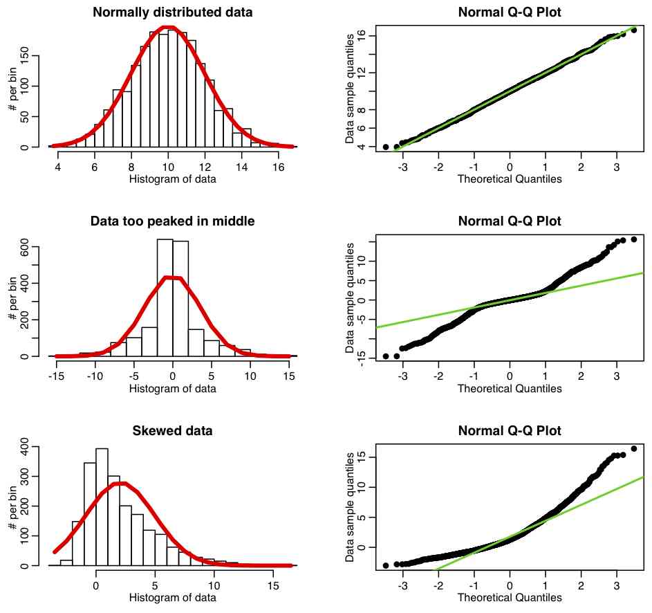
Now let’s look at the Chicago temperature data. The R script chicago_weather_b.R calls this function, and makes the following plot: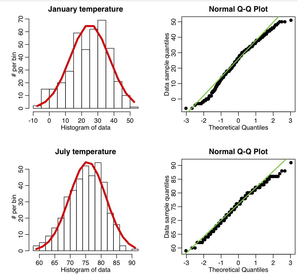
Central Limit Theorem: An interesting thing about the Normal distribution is that if we have a random sample of n points, X_i, drawn from *any* probability distribution (not just Normal), that has mean mu and std sigma, then if n is “large” the estimate of the sample mean will be Normally distributed about mu. The width of that Normal distribution will be sigma/sqrt(n). This is known as the Central Limit Theorem, and the quantity sigma/sqrt(n) is known as the standard error on the mean (SE). This implies that the larger the sample size of your measurements, the better your estimate of mu (because the width of the probability density for the mu estimate has width that is inversely proportional to n). What does “large” n mean; well around 10 and up is approximately considered “large”
The R script central_limit_example.R demonstrates this; it performs 10000 iterations where it generates samples of size 3 from the Exponential distribution (a one parameter distribution, with parameter lambda) with mean=1/lambda and variance=1/lambda^2. It calculates the sample mean and sample variance estimates for each of these sets of three points, and stores the results in a vector that it then histograms. It also repeats the process with samples of 10 and 30 points. It produces the following plot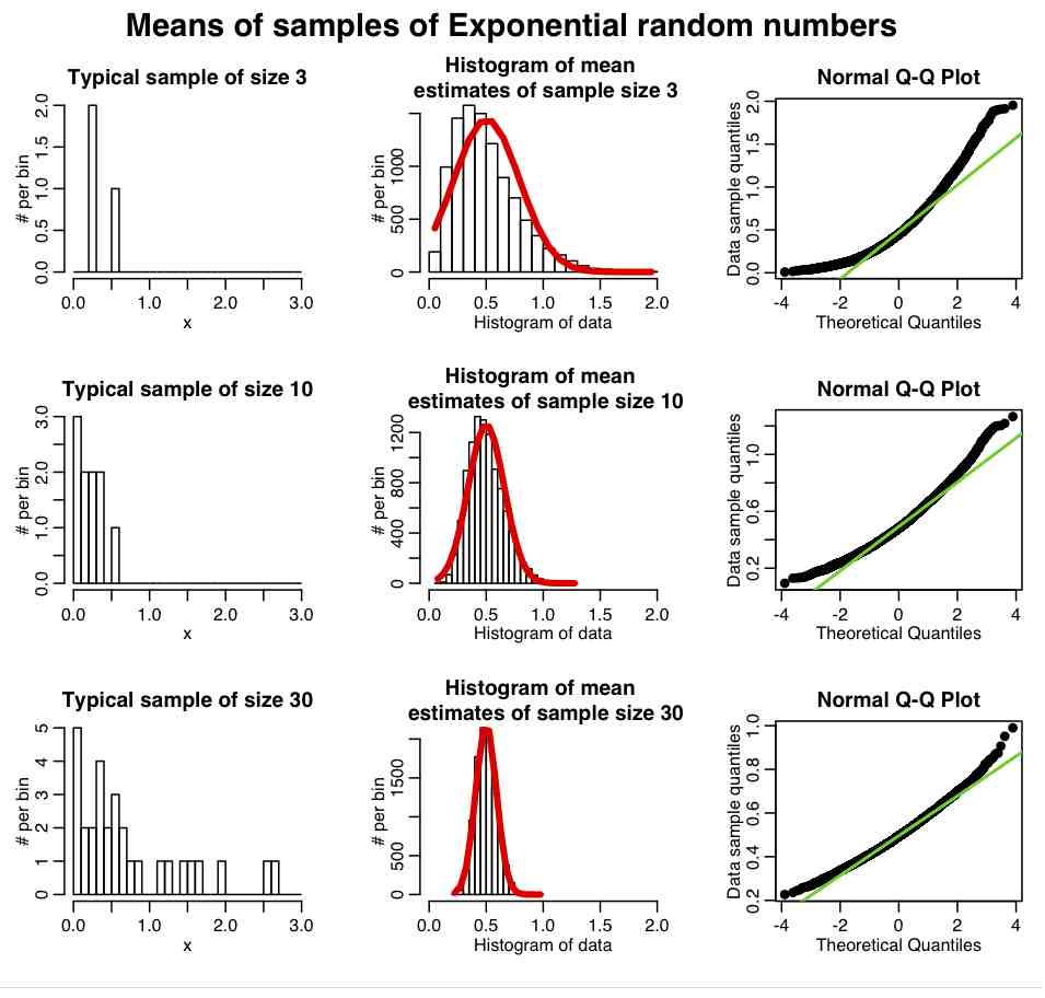
In reality, most data we wish to estimate the mean of are not Exponentially distributed. They are more or less Normally distributed. And it turns out that the central limit regime is reached much more quickly if the data are more-or-less normally distributed. The R script central_limit_example_b.R shows the same as above, except we sample the means of samples of Normally distributed random numbers with mean 1.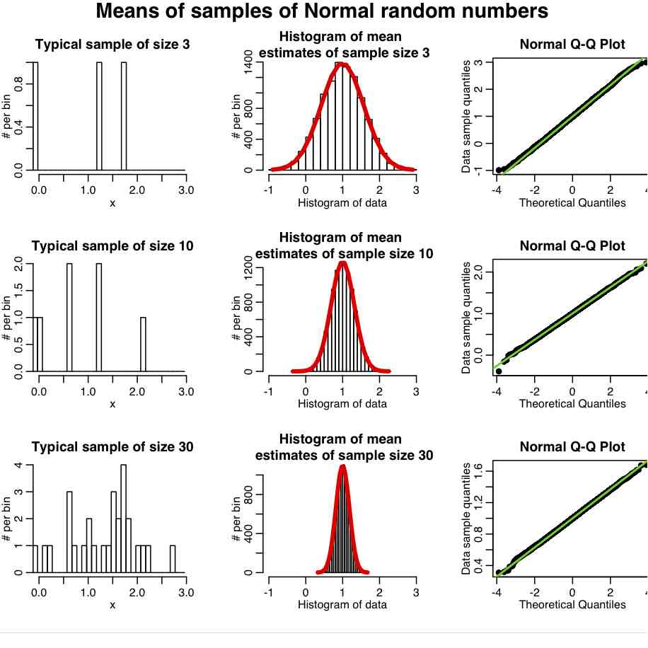
In general, the “pointier” the underlying probability distribution and the narrower the width, the quicker it reaches the central limit regime.
Central limit theorem applications: test if mean of large sample is consistent with some value: What does the central limit imply? Well, if our samples are large enough, we can assume that the mean is Normally distributed, and so we can use the Normal distribution to test whether the mean of a sample is consistent with being a particular value, or even whether or not two samples have different means. To test if the mean of the sample bar(X) is consistent with some value mu, we construct the statistic
 Equation (3)
where bar(X) is the sample mean and S is the sample standard deviation, so the denominator is the estimated standard error on the mean, which is S/sqrt(n). If the sample size, n, is large, the Central Limit Theorem tells us that the statistic Z should be distributed as a Normal distribution with mean 0 and standard deviation 1 if the null hypothesis is true (ie; that the mean of the sample truly was drawn from a Normal distribution with mean mu).
So we calculate the value of Z, and calculate its corresponding p-value under the assumption that Z~N(0,1). If p is very close to 1 or 0, we reject the null hypothesis.
Central Limit Theorem application: are the means of two large samples consistent with being drawn from distributions with the same mean: How about testing the hypothesis that two samples are consistent with being draw from probability distributions with the same mean? First we would construct the Z statistic in Equation (2) for the difference of the two means. Note that the sigma’s in that expression are equal to the estimates of the standard errors on the means. Under the null hypothesis that the underlying probability distribution means are equal, this Z should be distributed as Z~N(0,1). Again, we would calculate Z and assess the p-value.
Example: The R script central_limit_hypoth_test.R creates two samples, one randomly sampled from an Exponential distribution, and the other from a Uniform. It then calculates the means and standard erros of the distributions, calculates the Z statistic, and tests whether or not the value of Z is consistent with being drawn from N(0,1). The script produces the following plot (and also prints out the p-value):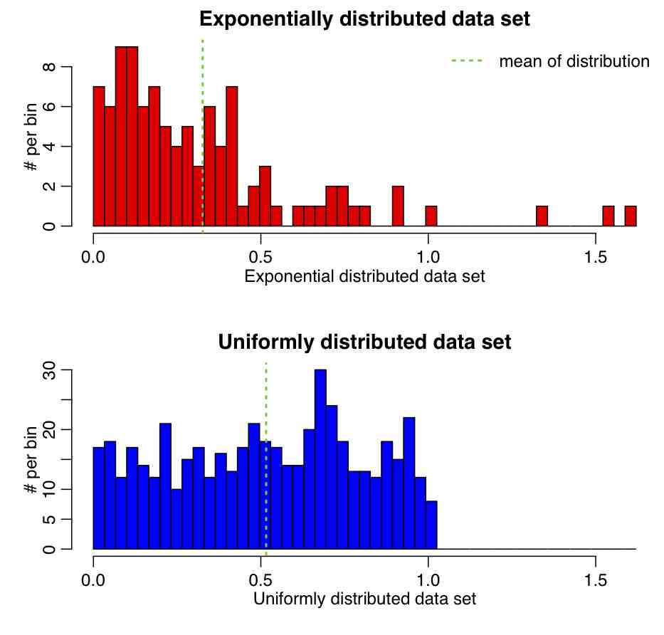
If we were to run this script 1000 times, how should the p-value be distributed?
Change the parameter of the Exponential distribution and the range of the uniform distribution and see how it affects the p-value.
Example: examine the output of the chicago_weather.R script and determine if this method can be applied to the means of the January and July temperatures. What is the p-value testing the hypothesis that the two means are drawn from the same distribution? Would you accept or reject the null? How about the January and February temperatures? And June and July temperatures? How about December 25th temperatures compared to December 24th temperatures.
If the sample sizes are small such that the central limit theorem does not hold, then somewhat more specialized methods need to be used, and here is where the Students-t distribution comes in…
Students-t distribution
Introduction:
The Student’s t-distribution comes in quite handy for, amongst other things, hypothesis testing whether or not a sample of Normally distributed data has a significantly different mean than the mean of another sample of Normally distributed data. Or, to test if the a sample of Normally distributed data has mean significantly greater or less than a particular value. The Student’s t-distribution is especially useful when the sample sizes are small (but can be used when the sample sizes are large, too).
From Wikipedia:
In the English-language literature [the test] takes its name from William Sealy Gosset‘s 1908 paper in Biometrika under the pseudonym “Student”.[8][9] Gosset worked at the Guinness Brewery in Dublin, Ireland, and was interested in the problems of small samples, for example [comparing] the chemical properties of [samples of] barley where sample sizes might be as low as 3. One version of the origin of the pseudonym is that Gosset’s employer forbade members of its staff from publishing scientific papers, so he had to hide his identity. Another version is that Guinness did not want their competitors to know that they were using the t-test to test the quality of raw material.[10]
Gosset was an Oxford educated applied mathematician and chemist. As an aside, in the early years of the 20th century Oxford went on to form one of the first programs in applied statistics, thanks to an endowment from Florence Nightingale, who was herself an unsung hero for her novel development and use of applied statistics in public health settings.
Anyway, we digress.
From Wikipedia:
In probability and statistics, Student’s t-distribution (or simply the t-distribution) is a family of continuous probability distributions that arises when estimating the mean of a normally distributed population in situations where the sample size is small and [the] standard deviation [of the underlying Normal distribution] is unknown. It plays a role in a number of widely used statistical analyses, including the Student’s t-test for assessing the statistical significance of the difference between two sample means, the construction of confidence intervals for the difference between two population means, and in linear regression analysis.
Probability density function: Just like the Normal distribution, the Student’s t-distribution is symmetric, but has heavier tails. The probability density function is

and has one parameter, nu>0, which is the number of degrees of freedom of the distribution. The mean of the distribution is 0. The variance of the distribution is nu/(nu-2), infinity for nu between 1 and 2, and otherwise is undefined. Notice that as nu gets very large, the variance gets close to 1.
R functions related to the Students-t distribution: The R function pt(n,nu) generates n random numbers from the Students-t distribution with nu degrees of freedom. The function dt(x,nu), pt(x,nu) return the PDF and CDF at x, respectively. It is the pt() function that you would use to assess a p-value testing the hypothesis that a number was drawn from that distribution.
Comparing Students-t distribution to Normal: The R script student_dist.R uses the dt(x,nu) function to create the following plot of the Student-t distribution for various values of nu, compared to a Normal distribution 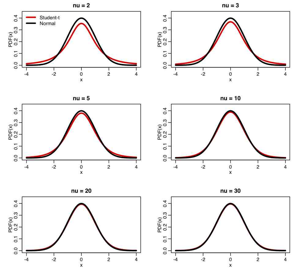
Students-t statistic: If we have n random numbers, x, drawn from a Normal distribution with mean mu and standard deviation sigma, then the statistic
 Equation(4)
is distributed as Students-t with degrees of freedom nu=(n-1), where bar(x) is the mean, and s is the sample standard deviation (sqrt of the sample variance). Take a look at Equation (3) and Equation (4); what is the difference? In both cases, what is the distribution underlying \bar{X}?
The R script student_t_example.R generates 10000 samples of two numbers each that are both drawn from the Normal distribution. The Students-t statistic is calculated for each sample, and the results histogrammed, and the Students-t distribution with nu=n-1=2-1=1 overlaid along with the Normal distribution for comparison. The script produces the following plot: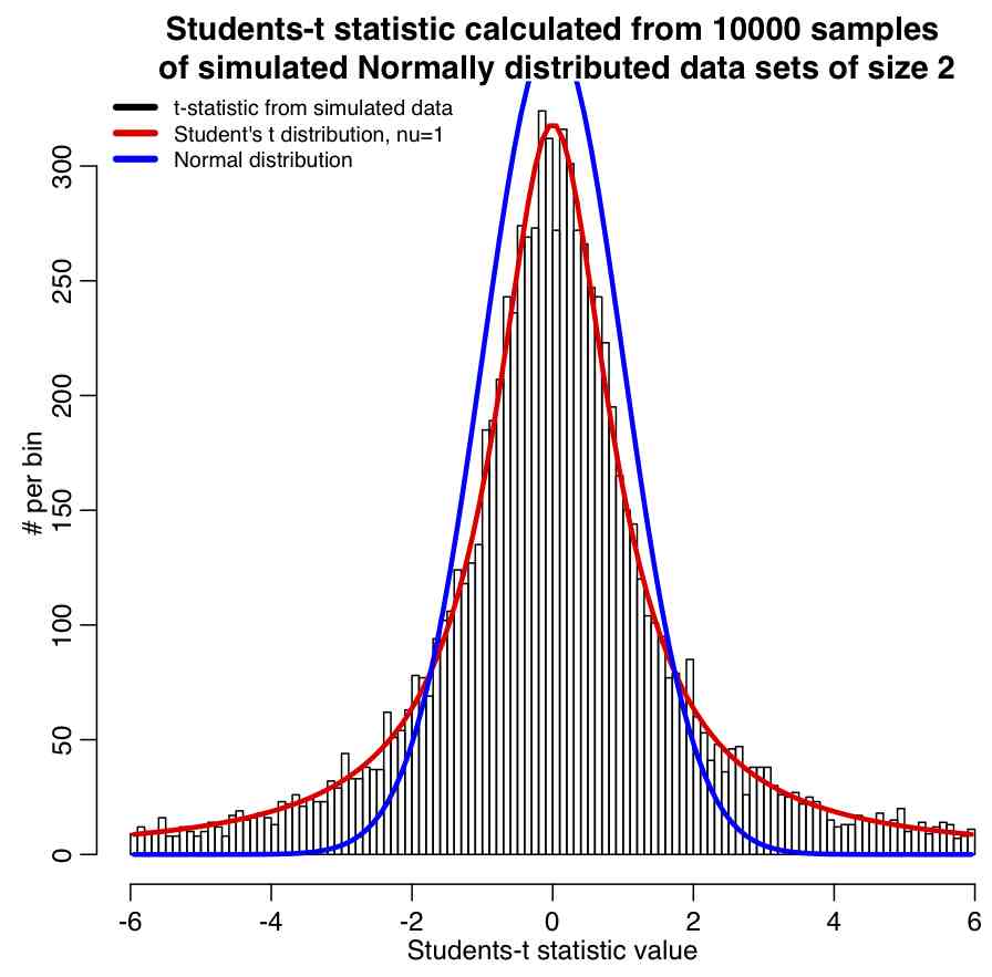
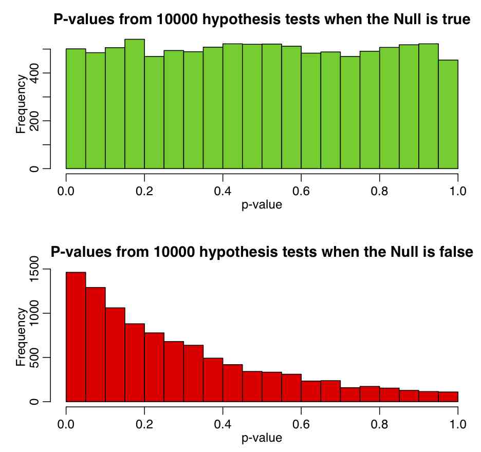
Using Students-t distribution to test hypothesis that the mean of a sample is consistent with some value: For a small sample of numbers, X_i, that are assumed to be drawn from the Normal distribution, we can test whether or not the mean of those numbers is consistent with some value mu, by forming the Student’s t-statistic of Equation 4, then used dt(t,df=length(X)-1) to calculate the p-value. If the mean of the numbers really is drawn from a distribution with mean mu, then the p-value will be Uniformly distributed between 0 and 1. The R script student_t_hypoth_test.R shows what happens when you generate 100000 samples of size 3, each drawn from a Normal distribution with mean 1. The top plot shows the Students-t p-value testing the Null hypothesis that mu=1, and the second shows the p-value testing the Null hypothesis that mu=1.5. One thing that needs to be noted again is that just because p<0.05 or p>0.95, the Null hypothesis is not necessarily untrue. The script produces the following plot:
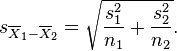
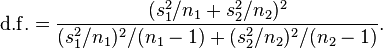
Using the Students-t distribution to test whether or not means of two samples are consistent with being equal: The independent two sample t-test tests whether or not the means of two samples, X1, and X2, of Normally distributed data appear to be drawn from distributions with the same mean. The test statistic is calculated as

with
The t-distribution of the test will have degrees of freedom
The script chicago_weather_c.R applies this test to determine if the temperatures on some day of the year have the same mean as the temperatures on another day of the year.
Limitations of using Student’s-t distribution for hypothesis testing of means: hypothesis testing of sample means with the Student’s-t distribution assumes that the data are Normally distributed. In reality, with real data this is often violated. When using some statistic (like the Students-t statistic) that assumes some underlying probability distribution (in this case, Normally distributed data), it is incumbent upon the analyst to ensure that the data are reasonably consistent with that underlying distribution; the problem is that the Students-t test is usually applied with very small sample sizes, in which case it is extremely difficult to test the assumption of Normality of the data. Also, we can test the consistency of equality of at most two means; the Students-t test does not lend itself to comparison of more than two samples.
Students-t for testing significance of correlation coefficients: The Students-t distribution underlies a hypothesis test that can be used to determine if the Pearson correlation statistic calculated for a paired sample of data is significantly different than zero. I won’t expect you to memorize how to apply the test, or even to apply it yourself; there is a nifty little tool available off of the Vassar college statistics pages that allows you to enter in the size of your paired sample, and the Pearson correlation statistic that you calculated. It then uses the hypothesis test to determine the p-value testing the hypothesis that the p-value is significantly different than zero. The “non-directional” p-value would be used when you have no prior expectation that X would be positively or negatively correlated to Y. It is also known as a two-tailed test. If you have some prior expectation that X would be positively or negatively correlated to Y (for instance, one would naively expect that weight and height would be positively correlated), you would use the directional p-value, which tests the significance of the correlation in one direction only.
In general, I err on the safe side (as far as getting analyses through review is concerned), and I don’t call a correlation “significantly” different than zero unless both the one-tailed and two-tailed tests have p<0.05.
In the R script chicago_pollution.R we calculated the Pearson correlation coefficient for temperature and ozone in Chicago between 2001 to 2012. With 4372 data points in our sample, we determined the correlation was 0.659. Is this significantly different than zero?
It should be noted that the hypothesis test that underlies the Pearson correlation statistic a priori assumes that the X and Y are Normally distributed. When this assumption is violated (particularly if it is badly violated), the p-values from this test are meaningless. There are other methods that can be used in those cases that essentially map the X and Y onto Normal distributions, and then assess the correlation coefficient.
From Wikipedia:
In probability theory and statistics, the chi-squared distribution (also chi-square or χ²-distribution) with k degrees of freedom is the distribution of a sum of the squares of k independent standard normal random variables. It is one of the most widely used probability distributions in inferential statistics, e.g., in hypothesis testing or in construction of confidence intervals.[2][3][4][5]
As we are about to see, if means from data in samples are Normally distributed (ie; the sample sizes are large enough that the Central Limit holds), the chi-square test enables us to test the hypothesis that the means of several samples are equal.
If Z1, …, Zk are independent, standard normal random variables, then the sum of their squares,

is distributed according to the chi-squared distribution with k degrees of freedom. This is usually denoted as
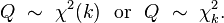
The chi-squared distribution has one parameter: k — a positive integer that specifies the number of degrees of freedom (i.e. the number of Zi’s)
Probability density function: The pdf of the chi-squared distribution is

where Γ(k/2) denotes the Gamma function. The mean of the distribution is k, and the variance is 2k.
R functions related to the chi-square distribution: The built-in R function rchisq(n,dof) generates random numbers drawn from the chi-square distribution with dof degrees of freedom. dchisq(Q,dof) is the value of the PDF at Q, and pchisq(Q,dof) is the CDF (and is used to test the significance of the Q statistic). Note that when the pchisq() function returns a value close to 1, that means the value of Q is much higher than would be typically expected under the null hypothesis. Thus, if (1-pchisq(Q,dof))<0.05, we would reject the null hypothesis that the Q statistic is consistent with being drawn from a chi-square distribution with dof degrees of freedom
Using chi-square distribution to test whether means of multiple samples are equal: An application of the chi-square distribution that we will use quite a lot is to test whether or not the means of several (say, m) samples are consistent with being drawn from the same value. To do this, first calculate the overall mean of all the samples combined. Let’s call this mu_est. Then, for each of the samples, calculate the mean and the standard error on the mean, bar(X) and SE, respectively. Now calculate the statistic

If the null hypothesis is true that the bar(X)_i are all equal to the overall mean, mu_est, then Q will be distributed as chi-squared with p degrees of freedom, where p=m-1 (we lose one degree of freedom calculating the overall mean). Recognize the quantity in the brackets as the Z statistic in Equation 3 above.
Note that when using this test, we implicitly assume that the sample sizes are big enough that we are in the regime where the Central Limit Theorem holds. If the means are calculated for small sample sizes, this test will return p-values that are wrong, and should not be used.
Using chi-square distribution to tests a hypothesis that the frequency distribution of certain events observed in a sample is consistent with a particular theoretical distribution: this is done with the Pearson chi-square test. Say we wanted to test if the number of murders observed per week day in Chicago between 2001 and 2012 was consistent with being uniformly distributed per weekday. We first calculate the total number of murders over the time period (call it N), and then determine the number of the N murders that fall on each of the 7 weekays days (call this N_i, where i goes from 1 to 7). Our expected Numbers are Nexpect_i (in this case the Nexpect_i are all equal to N/7). We then calculate the statistic
 Equation 5
where m is the number of bins (in this case, 7). This Q statistic will be distributed as chi-square with (m-1) degrees of freedom if the null hypothesis is true that the N_i are consistent with being equal to Nexpect_i. The R script chicago_pearson_chisq.R applies this test to determine if the murder data in Chicago are consistent with having no weekday dependence. The script produces the following plot: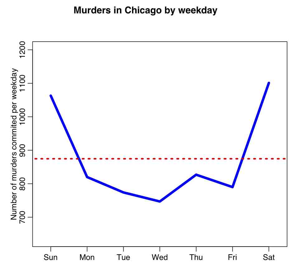
Cautions when using the Pearson chi-square test: One needs to keep in mind when using the Pearson chi-square test is that an underlying assumption (that is perhaps not often explicitly stated) of Equation 5 is that the test assumes that the stochasticity in the data is Poisson distributed (more on the Poisson distribution in a minute) and min(N_i) is large (ie; around, say, at least 10 to 30 or so), because as we are about to see when we discuss the Poisson distribution, this is the regime where N_i will be approximately Normally distributed. If min(N_i) is less than 10, this test should not be applied because it will not return accurate p-values.
There are also some subtleties to using this test that need to be kept in mind; for instance, if the data have trend in time and stochasticity, and we bin it by some repeating time period (like weekdays within a week), the data may appear to have significant weekday dependence, but that apparent weekday pattern has nothing to do with human preference or susceptibility to commit crimes on a certain day of week, but rather is just due to the overall trend. The R script trend_confounding.R shows an example of this using hypothetical daily data that I generated with linear trend with Normal smearing over a 10 year time period. There is no implicit weekday dependence when generating the data (ie; it is not periodic in weekday). The script produces the plot: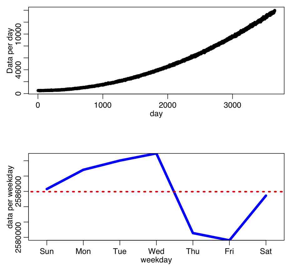
The script calculates the p-value testing the hypothesis that the data have no weekday dependence as p=4e-8, thus we would reject the null. When we get to the module that covers linear regression and factor regression, we will discuss how to take into account trend *and* possible dependence on weekday to truly test whether or not data have weekday dependence (or month-of-year, or day-of-year, or lunar phase, or whatever).
Poisson
Introduction: The Poisson distribution is one of the simplest of the discrete probability distributions. A discrete distribution can only produce random numbers that can assume only a finite or countably infinite number of values. In the case of the Poisson distribution, Poisson random numbers are drawn from integers from 0 to infinity. Because of this, the Poisson distribution often underlies the stochasticity in things we count. For instance, studies have shown that household size in many countries appears to be Poisson distributed. Also, number of children produced per woman in a society is close to being Poisson distributed.
Probability distribution: With the Poisson distribution, the probability of observing k counts when lambda is predicted is:
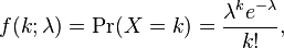
- The average value of random numbers drawn from the distribution is lambda, with standard deviation sqrt(lambda). Note that the Poisson distribution only has one parameter (lambda).
- The shape of the probability distribution f(k|lambda) for different values of lambda is
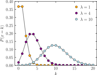
- Note that as lambda gets large, the Poisson distribution looks more and more symmetric. In fact, for lambda greater than about 10, the Poisson distribution approaches a Normal distribution with mean and variance both equal to lambda.

Poisson distribution and stochasticity of count data: Epidemic or population data usually consists of number of cases identified (counted) over some time period, like days, weeks, or months. Thus, as we will discuss later on, it is often assumed that the Poisson distribution underlies the stochasticity within each time bin.
What do we mean when we say that the Poisson distribution underlies the stochasticity within each time bin? It means that if we have a model (say, a model that posits that the number of counts over time rises linearly) that predicts that the average number of counts within that bin should have been lambda, then if the Poisson distribution underlies the stochasticity, the expected stochastic standard deviation within the bin would be sqrt(lambda).
In reality, with epidemic data that standard deviation within each bin is usually much larger than that predicted by the Poisson distribution because there are so many underlying causes of stochasticity in the spread of disease, from variations in population contact patterns, to variations in climate, etc etc. When the variation in the data is larger than expected, we say the data are over-dispersed. When discuss the Negative Binomial distribution below, we’ll talk about how it can address the over-dispersion problem.
Negative Binomial
The Negative Binomial distribution is one of the few distributions that (for application to epidemic/biological system modelling), I do not recommend reading the associated Wikipedia page.
Instead, one of the best sources of information on the applicability of this distribution to problems we will be covering here is this PLoS paper on the subject. As the paper discusses, the Negative Binomial distribution is the distribution that underlies the stochasticity in over-dispersed count data. Over-dispersed count data means that the data have a greater degree of stochasticity than what one would expect from the Poisson distribution.
Recall that for count data with underlying stochasticity described by the Poisson distribution that the mean is mu=lambda, and the variance is sigma^2=lambda. In the case of the Negative Binomial distribution, the mean and variance are expressed in terms of two parameters, mu and alpha (note that in the PLoS paper above, m=mu, and k=1/alpha); the mean of the Negative Binomial distribution is mu=mu, and the variance is sigma^2=mu+alpha*mu^2. Notice that when alpha>0, the variance of the Negative Binomial distribution is always greater than the variance of the Poisson distribution.
There are several other formulations of the Negative Binomial distribution, but this is the one I’ve always seen used so far in analyses of biological and epidemic count data.
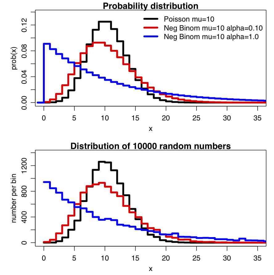
The PDF of the Negative binomial distribution is (with m=mu and k=1/alpha):
In the file negbinom.R, I give a function that calculates the PDF of the Negative Binomial distribution, and another function that produces random numbers drawn from the Negative Binomial distribution. The script produces the following plot:
Binomial Probability Distribution
The binomial distribution is the probability distribution that describes the probability of getting k successes in n trials, if the probability of success at each trial is p. Like the Poisson distribution, it is discrete. The probability mass function is
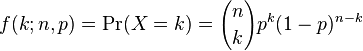
The probability function for various values of p and n looks like:
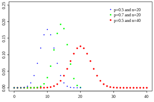
Notice that the distribution when p=0.5 and n=40 in the above plot looks almost Normally distributed. This is because when n*p>~10 or n*(1-p)>~10 the Binomial distribution approaches the Normal distribution with mean np and variance np(1-p).
Note that this means that if k>~10 or N-k>~10 the Normal approximation holds with mean k and variance k*(N-k)/N
Epidemic incidence data rarely reflect the true number of cases in the population, rather the data usually reflect the number that were identified by the surveillance system. For instance, the number of CDC confirmed influenza cases each week is only around 1/5,000 to 1/10,000 of the true number of cases in the population. This means that p for confirming influenza is quite small. It turns out that when n is large, and p is small, the number of successes is approximated by the Poisson distribution with lambda = n*p. This approximation is good if n ≥ 20 and p ≤ 0.05, or if n ≥ 100 and np ≤ 10
Example: say we had 5 groups of people (for instance, people in 5 different sections of an undergraduate calculus course), with N_i in each group (i=1,…,5) and N_tot=sum(N_i). We are told that k_i of the people in each group got at least a C grade on a midterm. We’d like to test the null hypothesis that the probability of passing the midterm was equal in each of the groups: ie that p=sum(k_i)/N_tot is the same underlying probability that the people in each group passed the midterm. Under the null hypothesis, the expected number in each group is thus k_expect=N_i*sum(k_i)/N_tot
If we are in the Normal regime (ie; the number observed to pass in each group is at least approximately 10) then we can test the null hypothesis that the expected number passing in each group is k_i^expect using the chi-square statistic
 Equation A
where m is the number of groups, and where sigma_expect is the std deviation uncertainty on k_expect:

If we are in the Poisson regime, such the N_i are all greater than around 100 and the k_i are all less than about 10 (it must have been a tough midterm!), then we would test the null hypothesis that the expected number passing in each group is k_i^expect using the chi-square statistic
 Equation B
If we test the null hypothesis that the probability of passing is the same in all groups, then we would estimate k_expect=sum(k_i)/sum(N_i), and the number of degrees of freedom for both of the chi-squares statistics above is (m-1). If the k_expect are instead particular values (not derived from the data), then the number of degrees of freedom is m.
Getting back to our example with 5 groups, say there were 250 people in each of the 5 sections of the Calculus class. In groups 1 through 5, the number of students passing the midterm were 125, 111, 98, 130, and 127 (which means that overall 591/1250=0.4728 of the students passed the midterm). We notice that the number of people who passed in each group is above 10, which means we can use the Normal approximation to test the null hypothesis that the probability of people passing was the same for all groups. We get that k_expect = 0.4728*250=118.2, and sigma_expect=sqrt(118.2*(250-118.2)/250)=7.89
Using Equation A, we get that Q = 11.899 with df=5-1=4. Using pchisq(Q,df) yields 0.9819, which yields the p-value testing the null hypothesis that the probability of passing the test was the same for people in all groups as p=1-0.9819=0.0181. We thus reject the null hypothesis.