[In this module, we will discuss the difference between mathematical and statistical modelling, using pandemic influenza as an example.  Example R code that solves the differential equations of a compartmental SIR model with seasonal transmission (ie; a mathematical model) is presented.  Also provided are an example of how to download add-on library packages in R, plus more examples of reading data sets into R, and aggregating the data sets by some quantity (in this case, a time series of influenza data in Geneva in 1918, aggregated by weekday).

Delving into how to write the R code to solve systems of ODE’s related to a compartmental mathematical model is perhaps slightly off the topic of a statistical modelling course, but worthwhile to examine; as mathematical and computational modellers, usually your aim in performing statistical analyses will be to uncover potential relationships that can be included in a mathematical model to make that model better describe the underlying dynamics of the system]

• Introduction
• Susceptible Infected Recovered (SIR) influenza model with periodic transmission rate
• The time-of-introduction of the virus is a parameter of the harmonic SIR model
• R code for SIR model simulation with harmonic transmission rate
• Example of aggregating a data set by some quantity

Introduction

Sometimes students who are new to applied mathematical modelling confuse mathematical models with statistical models, and vice versa.

With statistical models we can ask “does variable A appear to be related to variable B?”, then based on data for quantity A and quantity B, we develop a statistic that has an underlying probability distribution and we use that probability distribution to test whether or not A and B (appear!) to be related in a statistically significant way.

An example of a statistical model is the apparent dependence of the transmissibility of influenza on temperature and humidity; studies done with guinea pigs have shown that the probability that a guinea pig gets infected by an infected cage-mate is significantly related to temperature and humidity (in a non-linear way).

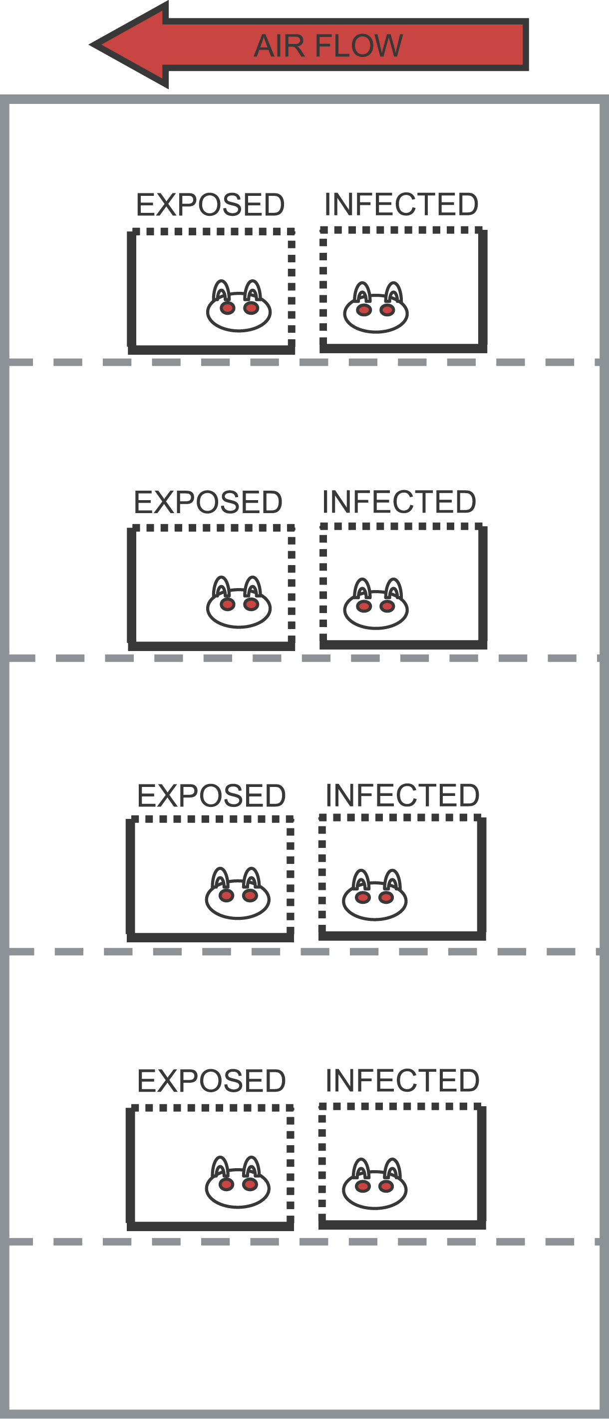
Low temperature and low humidity appear to make the influenza virus more transmissible, most likely by enabling the virus in the airborne droplets to survive longer and also perhaps by drying out the mucosal membranes, making it easier for the virus to invade the epithelial cells of the throat and nose.

In addition, studies of the severity of seasonal influenza epidemics have also shown that colder winters appear to be significantly associated with more severe flu seasons.

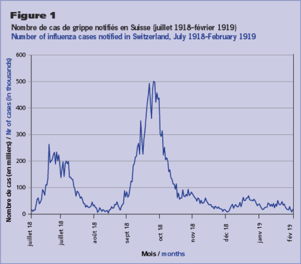
However this dependence on temperature doesn’t explain why in the 1918 and 2009 influenza pandemics exhibited a dual-wave-within-a-calendar-year structure, initiated by a summer wave.  If flu is most transmissible in cold weather, why would there be a big summer wave?

This is where mathematical models can help in our understanding of influenza transmission dynamics.  If we build a compartmental model for influenza that includes seasonality in transmission, it is quite adept at producing a dual summer wave.

What is a mathematical model?

As mentioned above, the equation for a statistical model has something on the LHS (let’s call it A), that is called the `dependent variable’.  On the RHS, you have a function that involves what are known as the `independent variables’.  Essentially the equation implies that variations in A depend on variations in the independent variables.  Of course, the equation that expresses these relationships is (by necessity) a mathematical equation.  But that does not make it a mathematical model, as we would normally think of it in the field of applied mathematics.

This is because life isn’t always so simple as the “thing X causes thing Y” approach. Sometimes you have interacting systems where a change in one aspect of the system is related to changes in another aspect, and vice-versa.

Take, for instance, a population of foxes and rabbits.  The foxes need to eat rabbits in order to produce young.  So the number of young each fox produces is a function of the number of rabbits.  But as the foxes eat the rabbits, the number of rabbits goes down, thus the rabbit death rate is related to the number of foxes.  There is no simple statistical equation that describes this interacting system because the number of rabbits depends on the number of foxes, and vice versa.  However, a set of mathematical equations known as the Lotka-Voltera model describes this kind of interacting system with a set of non-linear differential equations.  This is an example of a dynamical system.  And, more than that, the equations as written are an example of a deterministic dynamical system.  That means that if you start with the same inputs, you always get the same prediction for the number of foxes and rabbits over time.  Most sets of non-linear differential equations that describe deterministic differential equations have no analytic solution, and thus numerical methods must be used to solve the equations.

In reality, there is statistical variation around the expected values in the number of babies each fox has, and the number of rabbits each fox can kill.  An extension of such a model that takes this into account would be stochastic mathematical models, which can involve Stochastic Differential Equations, Markov Chain Monte Carlo, and Agent Based modelling.  The computational overhead in stochastic simulation of non-linear systems can be hefty.  Deterministic models are much faster to work with.

Game theory models or network models are also examples of models used by applied mathematicians.

An example of a deterministic mathematical compartmental model: The SIR model of disease transmission

With the SIR model, you start with a population of people who are susceptible to some infectious disease (say, influenza).  Initially a few infected people are added to the population and the entire population mixes homogeneously (meaning that the people an individual contacts each day are completely random).  During the duration of their illness the infectious people each infect on average X other people, who each then go on to and infect X other people, and so on, and so on, and so on.  Can you see that the number of infected people in the population will grow exponentially?  In fact, it can be shown that the exponential growth rate is equal to (X-1) divided by the length of the infectious period.

However, the exponential growth will eventually slow down, because the infected people recover and are now immune to the disease (in the SIR model, anyway… a model where they recover and then immediately become susceptible again is called a SIS model, and a model where people get infected and remain infected is an SI model); thus each infected person will still contact X other people during the course of their illness, but as time goes on a larger and larger fraction of the people they contact will be immune to the disease.  As this happens the spread of the disease slows, and eventually starts to decline.

X is a very special quantity.  Because it is the average number of people in a fully susceptible population that an infected person infects, it can be thought of as the number of infected people an infected person can reproduce.  In epidemiology, we thus refer to X as the Basic Reproduction Number (usually denoted by R0).  R0 is a fundamental quantity associated with disease transmission, and it is easy to see that the higher the R0 of a disease, the more people will ultimately tend to be infected in the course of an epidemic.

disease models like the SIR model involve population flow from one “compartment” (for instance, the “susceptible” compartment) to another compartment (for instance, the “infected” compartment.  Compartmental models like this are usually visualized with a diagram with boxes depicting each of the compartments, with arrows showing the flow between compartments:

The SIR model system of equations

The model equations giving the net rate of change of the fraction of the population in each compartment are (readers who have not yet been exposed to calculus can see a non-calculus description of how to implement an SIR model in this post):

Where “S”, “I”, and “R” are the number of people in the population that are susceptible, infected and recovered.  The parameter “beta” is known as the transmission rate, and is the contact rate times the probability of transmission of infection on contact. Each susceptible person contacts beta people per day, a fraction I/N of which are infectious; thus beta*S*I/N is the flow out of the susceptible compartment, and into the infected compartment. The transmission rate is the average rate of contacts a susceptible person makes that are sufficient to transmit infection.  The last part of that sentence is important, because not all contacts a person makes with an infectious person are the type of contacts that will lead to infection; for instance, flu can be spread with casual contact, but a disease like AIDS requires quite intimate contact, thus b for AIDS is much smaller than that of flu.   The parameter “gamma” is known as the recovery rate, and gamma*I is the flow out of the infected compartment, and into the recovered compartment.  The average time a person spends in the infected class is 1/gamma days, and is usually estimated from observational studies of infected people.  For flu 1/gamma is around 3 days.

Notice that the model in the above equations does not include births or deaths, immigration or emigration. It also assumes that the transmission rate is constant, which is probably not a good assumption for diseases like influenza which have a much higher incidence in the winter than any other time of year.

 

Susceptible Infected Recovered (SIR) influenza model with periodic transmission rate

For the discussion here, we will assume that the transmission rate of influenza has annual periodicity in temperate climates. Any periodic function can be expressed by an infinite sum of sines and cosines, so here we will make the simplifying assumption that the transmission rate is approximated by the first order harmonic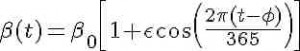
where beta_0 is the baseline transmission rate, epsilon is the relative seasonal forcing, and phi is the day of the year when the transmission rate is maximal.

The system of differential equations for the seasonally forced SIR model are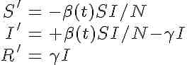
Note that, unlike the SIR model with a constant contact rate, we now have the time derivatives of S and I dependent on a function of time.  This is called a non-autonomous system of differential equations.  The mathematical analysis of non-autonomous disease models is much nastier than that of autonomous models, and the reproduction number is not straightforward to define.  In addition, there is no nice formula for the final size like we would be able to derive for the autonomous model with constant transmission rate.

The time-of-introduction of the virus is a parameter of the model

In fact the final size of the epidemic whose spread is described by the above equations is a function of the start time of the epidemic, relative to the day of the year when the transmission rate is maximal (I often refer to this as the time-of-introduction of the virus to the population).  We will see in a moment that the time-of-introduction can have a profound impact on the shape of the epidemic curve and final size of the epidemic.  This is certainly something that is not predicted by the statistical model!

R code for SIR model simulation with harmonic transmission rate

In the file sir_harmonic.R, I provide the code that will numerically solve the differential equations above, with different times-of-introduction of the virus to the population.  To run the script, you first must ensure that the deSolve library package has been installed in R on your computer.  To do this, type

install.packages("deSolve")

Then pick a mirror site close to your location.  The deSolve package is just one of many, many add-on library packages available in R.  As we progress through the course we will be downloading other library packages as needed.

Now download sir_harmonic.R to your R working directory, and type in the R console

source("sir_harmonic.R")

The following plot should be produced: 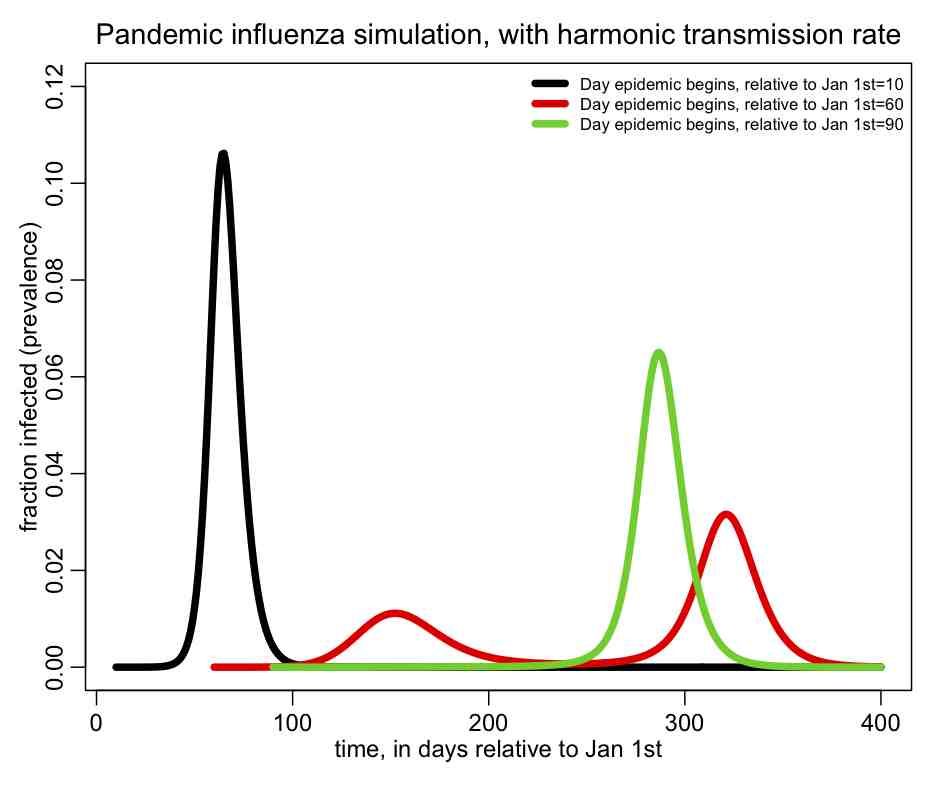You can see that the shape of the epidemic curve really depends on the time-of-introduction.  The R script also prints out the total fraction of the population that has been infected by the end of the epidemic, and you’ll notice that it too depends on the time-of-introduction.

I also show in the script a nice little trick in R to determine where local extrema occur in a time series, and in the script I used it to print out the times when the prevalence is at a minimum or maximum.

Example of aggregating a data set by some quantity

The file geneva.dat contains daily influenza-related hospitalizations in Geneva, Switzerland during the 1918 pandemic, obtained from Chowell et al, “Estimation of the reproductive number of the Spanish flu epidemic in Geneva, Switzerland”

The R script geneva.R, reads in this data and overlays the best fit SIR model with harmonic transmission rate (to run the script, you first need to download the R add-on libraries sfsmisc and chron). The fit of the parameters of the harmonic transmission SIR model to this data was performed by N.Zhang, I. Summer, and A.Murillo as part of their final project for the AML610 2013 spring semester course.  I modified their script to show the residuals of the fit (ie; the data minus the fit) aggregated by weekday, and to plot the results.  The script produces the following plot:

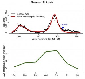In later modules, we will examine whether or not the residuals averaged-within-weekday are significantly different from one and other.