
In a past module, we examined how we could use methods in the R deSolve to fit the parameters of an SIR model to confirmed cases of influenza B in the Midwest region during the 2007-2008 flu season (the data were obtained from the CDC). In that module, we used a Least Squares goodness-of-fit estimator.
Refresher: the old R script for doing the fit with parameter sweeps
The comma delimited data file I prepared that contains CDC influenza data from the Midwest for the 2007-2008 season, is in midwest_influenza_2007_to_2008.dat
In the fit_example.R script I get the estimated incidence from an SIR model, with population size equal to the population of the Midwest, and assuming that one infected person is introduced into a completely susceptible population at time t0 (is this a good assumption?). The script assumes that t0 is week 44 of the year, and that the R0 of the epidemic is 1.35. I assume that the infectious period for flu is 1/gamma=3 days. In this example we assume that there is just one infected person at time t0, and that the population was fully immune. In reality, those initial conditions are also unknown model parameters that need to be estimated or the assumptions clearly stated.
The script produces the following plot: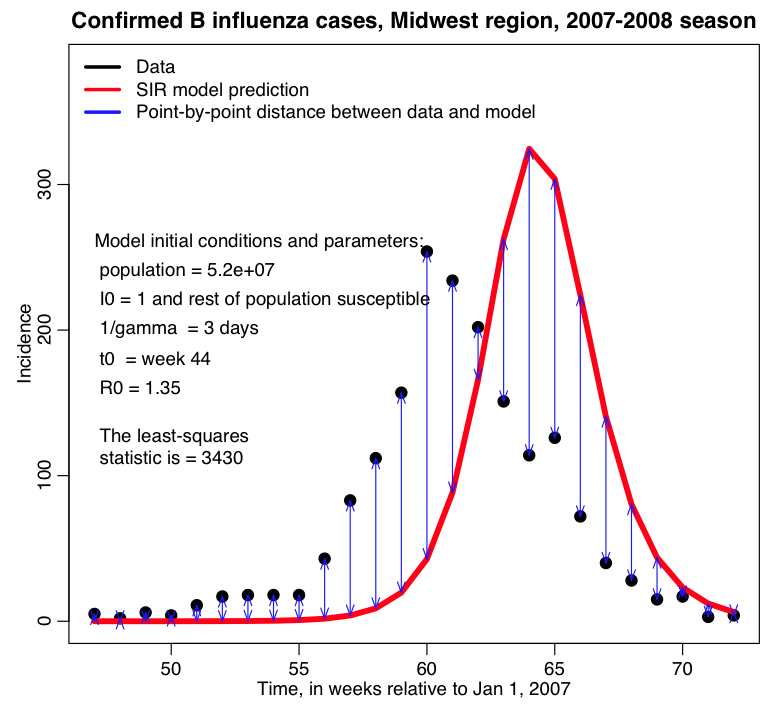
The values of R0 and t0 that I used in that script are clearly not ideal!
Rather than changing R0 and t0, and re-running the fit_example.R script many different times, it is much easier to write an R script to do a loop where it randomly samples many different hypotheses for R0 and t0 and calculates the least-squares statistic, keeping track of how the least squares statistic depends on R0 and t0.
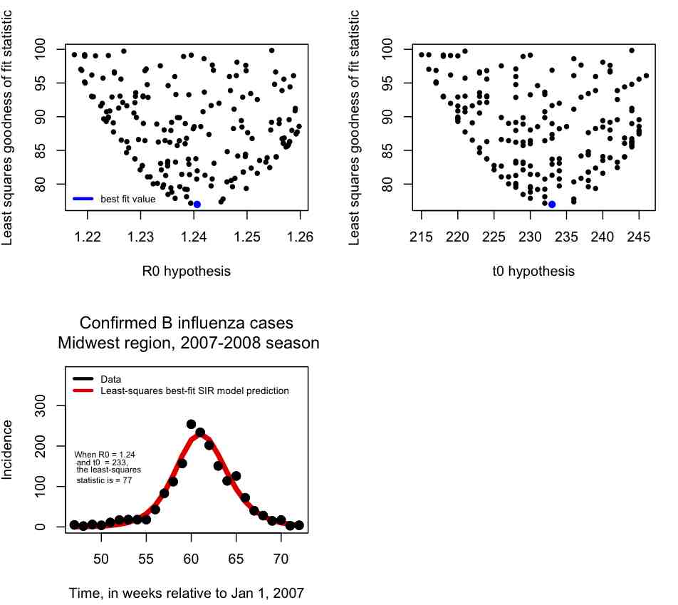
In blue I show the value of (R0,t0) that minimizes the Least Squares statistic, and then in the lower plot I overlay the best fit curve on the data. The fit looks quite reasonable.
In the file fit_iteration.R I provide the code that (eventually, after running a while) produces the above plots. Note that when you try this code out it will run slowly. This is because many, many different combinations of R0 and t0 had to be tried to get a good number of points in the plots, and a reasonable idea of what R0, t0 values will provide the best fit. The more parameters you fit for, the more parameter combinations you will have to try to populate plots like the ones above. In fact, the complexity of the process rises exponentially in the number of parameters.
A more sophisticated way: doing the parameter sweeps in C++ with utilities in the UsefulUtils and cpp_deSolve classes
A much faster way to do these fits is to write a C++ program to randomly sample parameter hypotheses, numerically solve the model under those hypotheses, and then calculate a goodness-of-fit statistic comparing the model to the data (this is especially fast if you have access to super-computing resources!)
In this past module, I introduced you to a C++ class, cpp_deSolve.h and cpp_deSolve.cpp, that I wrote that has a method SimulateModel to numerically solve systems of differential equations using the 4th order Runge-Kutta method. The class has hard-coded derivative equations for the SIR, SEIR, and harmonic SIR models; if you want a different model, you will have to code up the derivative equations yourself in the ModelEquations method.
Example of using the cpp_deSolve class to numerically solve an SIR model
In the file SIR_example.cpp, I give an example of an implementation of this class to numerically solve an SIR model. To compile and link the files, you can use the makefile makefile_solve by typing
make -f makefile_solve SIR_example
The program writes to standard output the temporal estimates of S and I and R. To run the file, and re-direct the results to a file called sir.out, type
./SIR_example > sir.out
Getting your data into your C++ program
Now, all the SIR_example.cpp program does is to numerically solve the model for just one set of parameter hypotheses. It also does not compare the model to data. In order to do the latter, we need some way of telling the program what the data values are. When running on a super-computing system, it is complicated to get a program to read a data file. Much better, if possible, is to have the data hard-coded in your C++ program itself.
I’ve thus created a class called FluData.cpp and FluData.h. The class contains the vector of time stamps and flu data for the Midwest B 2007-08 influenza data, filled in the constructor.
I didn’t type that data in there by hand, however! Instead I let R do it for me. In the R script midwest_flu_write_data.R I read in the Midwest influenza data, then, using cat() statements, I output that data in a format that I can simply copy and paste into my FluData.cpp constructor. The R script outputs the code to the file code_flu.txt
Putting it all together: parameter sweeps and calculating a goodness-of-fit statistic
In the C++ program Flu_example.cpp, I give an example of how to use the cpp_deSolve, FluData, and UsefulUtils classes (cpp_deSolve.h cpp_deSolve.cpp FluData.h FluData.cpp UsefulUtils.h UsefulUtils.cpp) to do parameter sweeps for beta and the time-of-introduction for an SIR model, and compare the incidence predicted by that model to the CDC Midwest 2007-08 B influenza data to calculate the Pearson chi-squared statistic. You can compile and link the files using the makefile makefile_flu