
In this past module, we discussed the various merits and applicability of the Least Squares, Pearson chi-square, Poisson likelihood, and Negative Binomial likelihood statistics.
And in this past module we discussed how we can use the graphical Monte Carlo method (aka fmin plus a half method) to determine the one-std deviation confidence interval on our parameter hypotheses when using a likelihood statistic, and we also discussed how the Least Squares and Pearson chi-square statistics can be converted to likelihood statistics.
As repeatedly discussed in this course, the Pearson chi-squared statistic is appropriate for count data that has enough counts per bin to be within the Normal approximation of the Poisson distribution (say, around approximately at least 10 counts per bin). It would be nice, however, if the Pearson chi-squared statistic could also reliably be used with over-dispersed count data.
Back in 1989, statisticians McCullagh and Nelder came up with a way to correct the Pearson chi-squared statistic for over-dispersion. Say the number of data points you are using in your model fit is N, and the number of parameters you are fitting for is k. Let’s also assume that in the random parameter sweep procedure we’ve been using for determination of best-fit model parameters we determine that the minimum value of the Pearson chi-squared, T, is Tmin. The dispersion corrected Pearson chi-squared statistic is
Tcorr = T*(N-k)/Tmin
Use this dispersion corrected statistic to determine the x-std deviation confidence intervals using the graphical Monte Carlo method. Recall that the Pearson chi-squared statistic can be converted into a negative log likelihood statistic simply by dividing it by two.
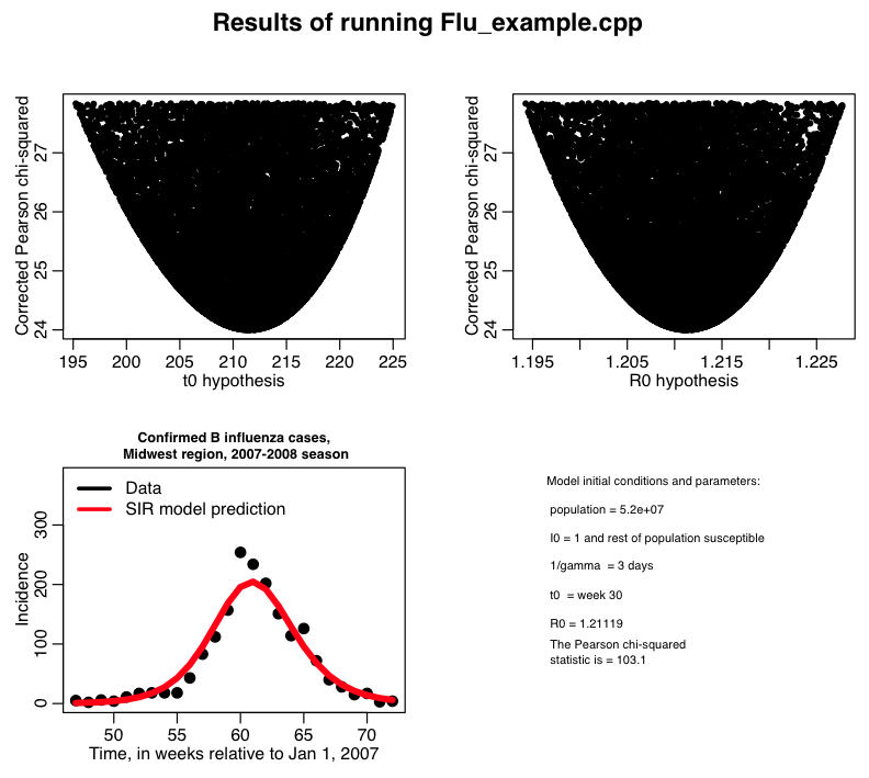
In this past module, we discussed using the Pearson chi-squared statistic to determine the best-fit parameters of an SIR model to influenza B data from the 2007-08 Midwest flu season. The results of random parameter sweeps fitting for the transmission rate beta, and the time-of-introduction of the virus to the population, t0, calculating the Pearson chi-squared statistic, T, can be found in the file flu_sim_b.out. The R script midwest_flu_b.R reads in this file and corrects the Pearson chi-square statistic for over-dispersion, and then obtains the 95% confidence interval on the parameter estimates. The script produces the plot:
Controlling the size of output files when doing parameter sweeps
In order to control the size of your output files when running in batch, it can be beneficial to only print out Pearson chi-squared or likelihoods that appear to be within 5std-dev of the current best-fit value (ie; f<(fmin + 25/2), if you are using a likelihood, T<(Tmin+25) if you are using Pearson chi-square). The C++ program Flu_example_b.cpp gives an example of doing this with our corrected Pearson chi-square statistic. You can compile and link it with the makefile makefile_flu.
Running Flu_example_b.cpp in batch on the ASU A2C2 ASURE super-computing cluster
In this past post, we talked about how to submit jobs to the ASU ASURE super-computing system. Copy the program Flu_example_b.cpp over to your working directory on the ASURE cluster and compile it using makefile_flu (ensure that you also have the UsefulUtils and cpp_deSolve and FluData class files in the same directory too) by typing
make -f makefile_flu Flu_example_b
You can use the batch submission script flub.sh to submit the job in batch. To submit 10 jobs in batch to run in parallel, type
sbatch --array=1-10 flub.sh
The output is directed to files of the form flu_b_xxx.out, where xxx is the job number. To concatenate the files into one, type
cat flu_b*.out >> temp.out
To copy the file temp.out to your local directory, type
scp <username>@hphn1.a2c2.asu.edu:~/flu/temp.out flu_sim_b.out
and you can then run the midwest_flu_b.R script to get the plots above.