[After reading this module, students should be familiar with probability distributions most important to modelling in the life and social sciences; Uniform, Normal, Poisson, Exponential, Gamma, Negative Binomial, and Binomial.]

Contents:
Introduction
Probability distributions in general
Probability density functions
Mean, variance, and moments of probability density functions
Mean, variance, and moments of a sample of random numbers
Uncertainty on sample mean and variance, and hypothesis testing
The Poisson distribution
The Exponential distribution
The memory-less property of the Exponential distribution
The relationship between the Exponential and Poisson distributions
The Gamma and Erlang distributions
The Negative Binomial distribution
The Binomial distribution

Introduction

There are various probability distributions that are important to be familiar with if one wants to model the spread of disease or biological populations (especially with stochastic models).  In addition, a good understanding of these various probability distributions is needed if one wants to fit model parameters to data, because the data always have underlying stochasticity, and that stochasticity feeds into uncertainties in the model parameters.  It is important to understand what kind of probability distributions typically underlie the stochasticity in epidemic or biological data.

Probability distributions in general

Probability density functions

In probability theory, the probability density function is the function of a random variable that describes the probability that the random variable can assume a specific value (for a discrete probability distribution, the term probability mass function is used). You will often hear me refer to probability density and mass functions as “probability distributions”.

There are several probability distributions that are used, either explicitly or implicitly, in epidemic and biological modelling.  For instance, the Exponential distribution is often used to describe the probability distribution of time spent in an state, such as th.  The Gamma distribution is also used for this purpose.  The Normal, Poisson, and Negative Binomial distributions are used to describe the stochasticity in epidemic incidence data.  The Uniform distribution can be used for a variety of purposes, one of which we will discuss below.

Mean, variance, and moments of probability distributions, with Uniform and Normal distributions as examples

If f(x) is the probability function for some continuous probability distribution, then the moments of the distribution are defined as:

The mean is the first moment, and the variance of the distribution is given by

One of the simplest probability distributions (conceptually at least) is the Uniform probability distribution with probability density:

The probability density looks like:

Notice that all intervals of the same length on [a,b] are equally probable.
It is easy to show from the moments formula that the mean and variance of the Uniform distribution are 0.5(a+b) and (b-a)^2/12, respectively.

The Normal (or Gaussian, or bell curve) distribution is also very commonly encountered. It has the probability density function

Notice that the PDF is symmetric about mu.  It is straightforward to show that the mean and variance of this distribution are mu and sigma^2.

For various values of mu and sigma, the distribution looks like this:

Note that the distribution is symmetric about mu, and the larger sigma is, the broader the distribution is.

Many probability distributions approach the Normal distribution under certain conditions, and we will discuss this further as we discuss the various probability distributions later in this module.

Mean, variance, and moments of a sample of random numbers

Given a distribution of n random numbers, X_i, the estimated sample mean is

The k^th sample moment is given by

Akin to the definition of the variance of a probability distribution given above, the sample variance is

Uncertainty on sample mean and variance, and hypothesis testing

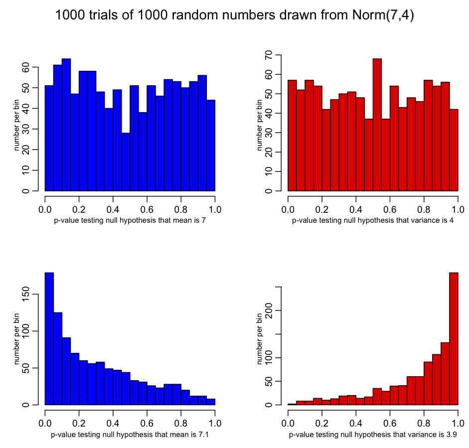
Let’s assume that the random numbers X_i are drawn from some probability distribution with true mean mu, true variance sigma^2, and moments calculated with the formulas above.  Because we only have a finite number of observations (n) in the data, our estimated sample mean and variance are imperfect estimates of the true mean and variance; finite sample size means that there is a stochastic element to our estimate of the mean and variance.If n is fairly large (say, greater than 100 or so), probability theory tells us that the estimated mean of the distribution is Normally distributed about the true mean, with variance

Why am I providing formula for the variance of the sample mean? Because when you calculate a sample mean, it is good to know what your uncertainty on that estimate is.  If you have very little data (small n), and/or broadly distributed data (large sigma), the uncertainties on the sample mean can be substantial, and you need to be aware of that if you want to compare what you see in your data to what others observed in their data (ie; if you want to test the null hypothesis that the average you observe in your data is consistent with that observed in another similar data set, and/or is consistent with the mean of some known probability distribution).

pnorm( (S-T)/sqrt(var_S) )

The file random_norm.R gives an example of testing the hypotheses that mean and variance of a sample (in this case, a sample of 1000 random numbers drawn from the Normal distribution) are consistent with some value.  The script does 1000 trials of generating random samples, and calculates the p-value for each trial for the hypothesis tests on the mean and variance.  The script produces the following plot:

Poisson distribution:

The Poisson distribution is one of the simplest of the discrete probability distributions, having only one parameter, the mean, lambda. A discrete distribution can only produce random numbers that can assume only a finite or countably infinite number of values.  In the case of the Poisson distribution, Poisson random numbers are drawn from integers from 0 to infinity.  Because of this, the Poisson distribution often underlies the stochasticity in things we count.  For instance, studies have shown that household size in many countries appears to be Poisson distributed.

With the Poisson distribution, the probability of observing k counts when lambda are predicted is:

The average value of random numbers drawn from the distribution is lambda, with standard deviation sqrt(lambda).  Note that the Poisson distribution only has one parameter (lambda).
The shape of the probability distribution f(k|lambda) for different values of lambda is

Note that as lambda gets large, the Poisson distribution looks more and more symmetric about lambda.  In fact, for lambda greater than about 10, the Poisson distribution approaches a Normal distribution with mean and variance both equal to lambda.
Epidemic data usually consists of number of cases identified (counted) over some time period, like days, weeks, or months.  Thus, as we will discuss later on, it is often assumed that the Poisson distribution underlies the stochasticity within each time bin.

What do we mean when we say that the Poisson distribution underlies the stochasticity within each time bin?  It means that if we have a model (say, an SIR model) that predicts that the average number of counts within that bin should have been lambda, then if the Poisson distribution underlies the stochasticity, the standard deviation of the expected stochastic variation within the bin would be sqrt(lambda).

In reality, with epidemic data that standard deviation within each bin is usually much larger than that predicted by the Poisson distribution because there are so many underlying causes of stochasticity in the spread of disease, from variations in population contact patterns, to variations in climate, etc etc.  When the variation in the data is larger than expected, we say the data are over-dispersed.  When discuss the Negative Binomial distribution below, we’ll talk about how it can address the over-dispersion problem.

Exponential distribution

Deterministic compartmental models like the simple Susceptible, Infected, Recovered (SIR) model have the inherent underlying assumption that the time spent in each state is exponentially distributed.

The exponential distribution is continuous, and defined on the positive real numbers.  It has one parameter, lambda. The probability of spending time x in a state, given average rate to leave the state, lambda, is

The average and standard deviation of the Exponential distribution are both 1/lambda. The probability distribution for  f(x|lambda) looks like

Now let’s return back to the Exponential distribution and its connection to compartmental modelling.  Let’s assume that we have an SIR model with recovery rate gamma from the infectious class. If the recovery rate is gamma, the probability distribution for the time spend in the infectious period is

P(t)=gamma*exp(-gamma*t).

Note that the most probable time for leaving the infectious stage is t=0!  This is rather unrealistic, and there are ways to incorporate more realistic probability distributions for the infectious stage in a deterministic compartmental model that I will discuss in a later post.

Memoryless property of exponential distribution

Let’s calculate the probability that an infected individual will recover between times t to t+delta_t (refer to this as event “A”), given that the individual has been infected up until time t (refer to this as event “B”).  Baye’s theorem tells us that

P(A|B) = P(B|A)P(A)/P(B)

It should be easy to see that P(B|A)=1 because A occurring necessarily implies that B must have occurred too.  We also can easily calculate, by integrating the probability distribution, that

P(A) = (1-exp(-gamma*delta_tt))*exp(-gamma*t), 
and 
P(B) = exp(-gamma*t).

Thus

P(A|B) = 1-exp(-gamma*delta_t)

Notice that this does not depend on time!  The probability of leaving the infectious state is constant in time, and does not depend on how long an individual has been infectious.  This is know as the “memoryless” property of the exponential distribution.

More realistic probability distributions for the infectious stage (like the Gamma distribution) are not memoryless; the probability of leaving a class in some time step depends on how long the individual has so far sojourned in that class.  We will talk about the Gamma distribution further down in this module.

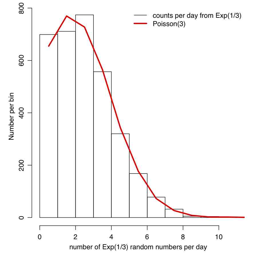
Relationship between Exponential and Poisson distributions

It turns out that the Exponential and Poisson distributions are intimately related (perhaps the fact that they are both one parameter distributions, both with a parameter normally referred to as “lambda”, hints at that?).  The Exponential distribution describes the time between events in a Poisson process.  For instance, assume that lambda babies are on average born in a hospital each day, with underlying stochasticity described by the Poisson distribution.  It can be shown that the probability distribution for the wait time (in days) between babies is lambda*exp(-t*lambda)

Similarly, if we have an Exponential process with probability distribution (lambda)exp(-t*lambda), the number of events that occur in some fixed unit of time, elta_t, is Poisson distributed with mean (lambda*delta_t)

The R file random_pois_and_exp.R demonstrates this connection between the Poisson and Exponential distributions (and also demonstrates how to set a random seed in R).  The file produces the plot:

The Gamma Distribution

As mentioned above, an underlying assumption of a compartmental disease model is that the probability distribution for the time spent in the compartment is Exponentially distributed.  And, as seen above, this implies that the most probable time to leave that compartment is at t=0.  This is obviously highly unrealistic in many cases, such as in the case of a model compartment that correspond to a disease state.

A distribution that gives a much more realistic description of the time spent in a disease state is the Gamma distribution, which is based on two parameters; the shape parameter, k, and the scale parameter, theta.  When the shape parameter is an integer, the distribution is often referred to as an Erlang distribution.

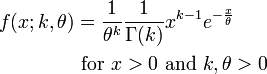
The PDF of the Gamma distribution is

For various values of k and theta the probability distribution looks like this:

Notice that when k=1, the Gamma distribution is the same as the Exponential distribution with lambda=1/theta

When k>1, the most probable value of time (“x” in the function above) is no longer 0.  This is what makes the Gamma distribution much more appropriate to describe the probability distribution for time spent in a disease state.
Erlang distributed probability distribution for the sojourn time can be incorporated into a compartmental disease model in a straightforward fashion; for instance, assume that the sojourn time in the infectious stage of an SIR model is Erlang distributed with k=2 and theta = 1.5 (with 1/gamma = k*theta)… simply make k infectious compartments, each of which (but the last) flows into the next with rate gamma*k.  The last compartment flows into the recovered compartment.

Negative Binomial distribution

The Negative Binomial distribution is one of the few distributions that (for application to epidemic/biological system modelling), I do not recommend reading the associated Wikipedia page.

Instead, one of the best sources of information on the applicability of this distribution to problems we will be covering here is this PLoS paper on the subject:  Maximum Likelihood Estimation of the Negative Binomial Dispersion Parameter for Highly Overdispersed Data, with Applications to Infectious Diseases  As the paper discusses, the Negative Binomial distribution is the distribution that underlies the stochasticity in over-dispersed count data.  Over-dispersed count data means that the data have a greater degree of stochasticity than what one would expect from the Poisson distribution.

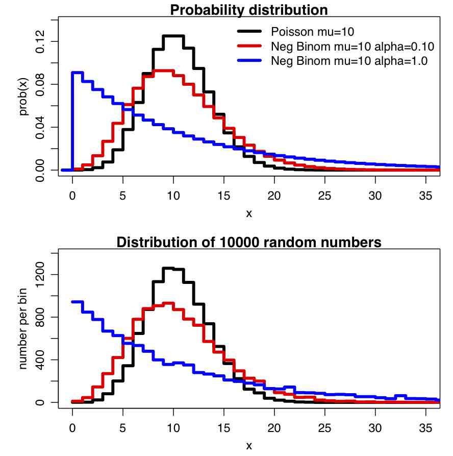
Recall that for count data with underlying stochasticity described by the Poisson distribution that the mean is mu=lambda, and the variance is sigma^2=lambda.  In the case of the Negative Binomial distribution, the mean and variance are expressed in terms of two parameters, mu and alpha (note that in the PLoS paper above, m=mu, and k=1/alpha); the mean of the Negative Binomial distribution is mu=mu, and the variance is sigma^2=mu+alpha*mu^2.  Notice that when alpha>0, the variance of the Negative Binomial distribution is always greater than the variance of the Poisson distribution.

There are several other formulations of the Negative Binomial distribution, but this is the one I’ve always seen used so far in analyses of biological and epidemic count data.

The PDF of the Negative binomial distribution is (with m=mu and k=1/alpha):

In the file negbinom.R, I give a function that calculates the PDF of the Negative Binomial distribution, and another function that produces random numbers drawn from the Negative Binomial distribution.  The script produces the following plot:

Binomial distribution

The binomial distribution is the probability distribution that describes the probability of getting k successes in n trials, if the probability of success at each trial is p.

Epidemic incidence data rarely reflects the true number of cases in the population, rather it reflects the number that were identified.  For instance, the number of CDC confirmed influenza cases each week is only around 1/5,000 to 1/10,000 of the true number of cases in the population.  This means that p for confirming influenza is quite small.  It turns out that when n is large, and p is small, the number of successes is approximated by the Poisson distribution with lambda = n*p.

Homework #2; due at 4pm Thus Feb 14th.
R code for solutions hwk2_solutions.R
Doc file with solutions AML610_hwk2_solutions.docx