
In this module students will compare the performance of several fitting methods (Least squares, Pearson chi-squared, and likelihood fitting methods) in estimating the rate of exponential rise in initial epidemic incidence data. Students will learn about the properties of good estimators (bias and efficiency).
A good reference source for this material is Statistical Data Analysis, by G.Cowan
Another good reference source (in a very condensed format) for statistical data analysis methods can be found here.
Contents:
Introduction
Properties of good estimators
Generating simulated exponential rise data
Estimation of the rate of exponential rise: Least Squares
Estimation of the rate of exponential rise: Pearson chi-squared
The Poisson maximum likelihood method
Estimation of parameter confidence intervals: any maximum likelihood method
Estimation of the rate of exponential rise: Poisson maximum likelihood method
Testing for over- or under-dispersion.
Correcting for over- or under-dispersion
Better method for determination of parameter estimates and their covariance when using the Pearson chi-squared method
When a new infectious disease begins spreading in the population and appears to pose a significant threat to public health (like SARS or pandemic influenza), the race is on for public health officials to determine the basic reproduction number, R0, because it indicates how many people each infected person will infect (and thus indicates how large the epidemic might be). R0 can be deduced from tracing of contacts of infected people early in the epidemic, but this process is time consuming and fraught with difficulties. A more straightforward means to determine R0 is to determine the rate of exponential rise in cases at the beginning of the epidemic, and then calculate R0 using whatever disease model likely best describes the disease (for instance, some diseases can be described with an SIR model, but many diseases have a long exposed-but-not-yet-infectious period, and a model like an SEIR model that includes an Exposed class would be more appropriate… however, keep in mind that all of these compartmental infectious disease models all have an exponential rise that is some function of R0).
In this model we will be discussing the performance of various fitting methods (Least squares, Pearson chi-squared, and likelihood methods) when fitting for the rate of exponential rise in epidemic incidence data.
Properties of good estimators (from any fitting method)
Whatever fitting method one uses to estimate model parameters, we want the 95% confidence interval on the model estimates to contain the true value of the parameter 95% of the time. In order for this to occur, the parameter estimate has to be unbiased, and the estimated uncertainty on the parameter estimate has to be efficient.
One way to tell if a fitting method produces unbiased and efficient estimates is to do what are called simulated data studies (aka Monte Carlo studies). For simplicity, I’ll describe this process for a model that has only one parameter to be estimated, theta. Generate M simulated data sets with theta=theta_true; let’s assume this is simulated epidemic incidence data. Randomly smear the incidence data in each time bin about the predicted value with random numbers drawn some probability distribution (for instance, the Poisson distribution, or Negative Binomial distribution). Then, for each of the M simulated data sets, use your fitting method of choice to estimate the parameter theta, theta_est, and its one standard deviation uncertainty, delta_theta. Below we will be discussing Least-squares, Pearson chi-squared, and likelihood fitting methods. If the fitting method returns unbiased and efficient estimates, the distribution of (theta_true-theta_est)/delta_theta should be Normally distributed, with mean consistent with 0, and variance consistent with 1. If the mean is not consistent with zero, the parameter estimate is biased. If the variance is greater than 1, then the estimates of delta_theta are too small.
Generating simulated exponential rise data
The R script generate_exponential_rise.R generates 250 samples of simulated weekly incidence data on the exponential rise of an influenza pandemic with R0=1.5 and recovery rate gamma=1/5 days^(-1). Recall that for an SIR model, the rate of exponential rise is rho=gamma*(R0-1).
The epidemic data are aggregated into bins of a week, thus the model prediction for a bin that ends at time t_i is

where delta_t is the time span of the bin. This yields the predicted value is:

In the script, the data in each bin are randomly smeared about the predicted value with an Negative Binomial distribution with mean mu=y_pred and alpha=0.2
Note that when we wish to compare y_pred to data for any of the fitting methods, we need to normalize y_pred such that its sum over all bins equals the sum of the data. Thus we need y_pred_normalized = y_pred*sum(y_data)/sum(y_pred).
Can you see that in the case of an exponential, this means we only have to fit for rho, and not a?
The script also generates simulated data smeared with random numbers drawn from the Poisson distribution with lambda=y_pred
The script outputs the simulated data into simulated_exp_R15_alpha02_nb.txt and simulated_exp_R15_pois.txt for the NB and Poisson smearing, respectively. The columns of the files correspond to the different simulation runs. These data will be used below when we discuss the Least Squares, Pears chi-squared, and likelihood fitting methods.
The script produces the following plot for the simulated data smeared with the Negative Binomial: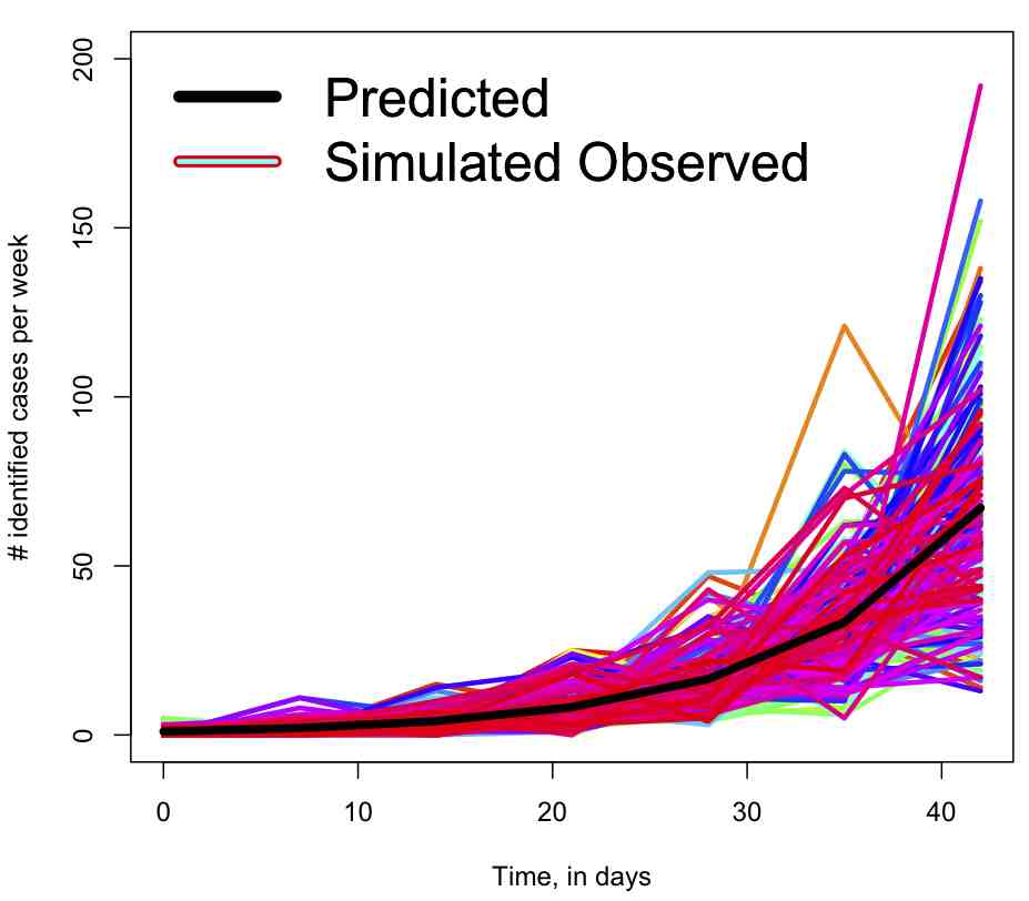
Estimation of the rate of exponential rise: Least Squares
In an earlier module, I discussed model parameter estimation using the Least Squares method. I mention in that post that the LS method has the underlying assumption that the stochasticity within each bin is exactly equal. For data in the epidemic rise, this is not usually a good assumption; if we assume underlying Poisson or Negative Binomial stochasticity, bins very early on in the rise will have much larger relative stochasticity than bins further into the rise. For this reason, we might expect that the Least Squares method will produce bias and inefficient estimators of the rate of exponential rise. But does it? Let’s find out…
The R script fit_exp_with_LS.R reads in the simulated data sets generated above, and uses the R lm() function to use a Least Squares method to fit a straight line to the logarithm of the simulated data in each of the 250 data sets. It stores the estimated rate of rise, and uncertainty on the estimate in vectors, then it calculates normalized residuals
n=(rho_est-rho_true)/delta_rho_est
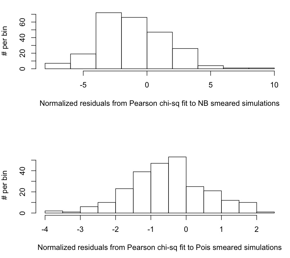
It does this for both the data sets that were generated with Negative Binomial random smearing, and Poisson random smearing. The script outputs the following plot: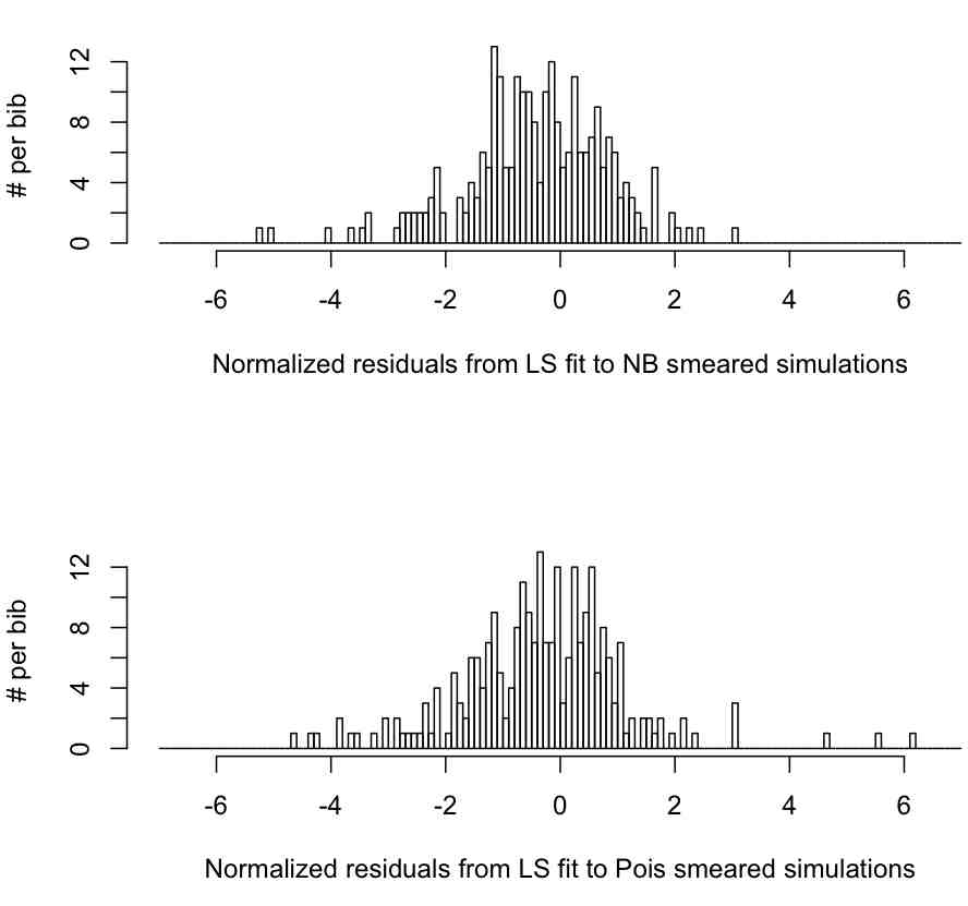
Based on the output of the script, is the mean of n consistent with zero, and is the variance consistent with 1?
Well, the script tells us that for the 250 data sets smeared with the NB, the mean of n is mu=-0.42, with standard deviation sigma=1.24, and we need to test the null hypotheses that the mu=0, and sigma=1. To do this, we need to know the uncertainty on our estimates of mu and sigma. We have previously discussed in an earlier module that the Central Limit Theorem tells us that the uncertainty on the mean of a distribution is delta_mu=sigma/sqrt(N), with underlying Normal stochasticity. In addition, the uncertainty on sigma is delta_sigma=sigma/sqrt(2N) (see section 36.1.1 of this reference)
Now, the sum of the squares of k Normally distributed random variables is distributed as chi-squared with dof=k (see here). If we wish to test the hypothesis that the mean is 0, we will have one Normally distributed random variable S=(mu-0)/delta_mu. Thus we wish to test the hypothesis that S^2 is consistent with the chi-squared distribution with one degree of freedom. You can do this in R with the pchisq() function:
p-value=1-pchisq(S^2,1)
Try
y=rnorm(10000)
hist(1-pchisq(y^2,1))
which will produce the plot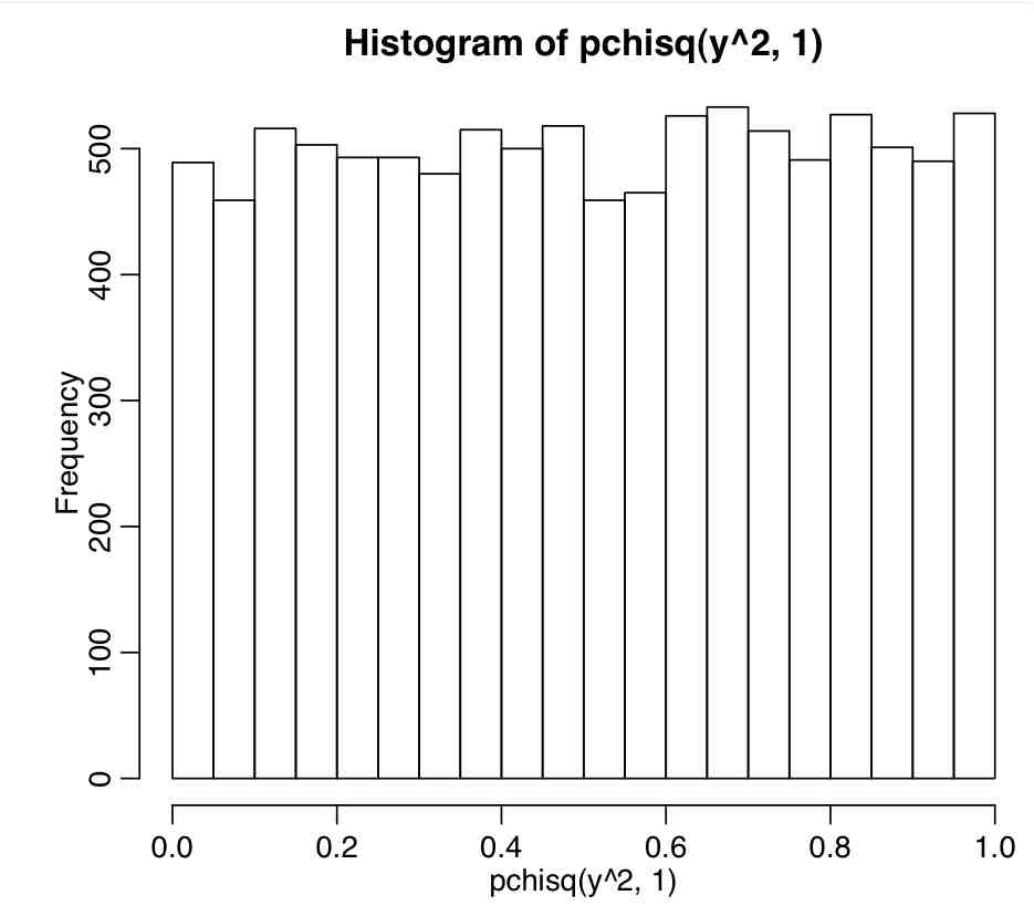
Note that pchisq(S^2,1) it is uniformly distributed when S is Normally distributed with mean 0 and variance 1. This is what we expect…. 5% of the time, by mere random chance, the p-value will be less than 5% when the random data is drawn from the same distribution as the null hypothesis.
Getting back to the results of our simulations, the script tells us that for the 250 data sets smeared with the NB, the mean of n is mu=-0.42, with standard deviation sigma=1.24. Thus, we get delta_mu=1.24/sqrt(250)=0.08, and delta_sigma=sigma/sqrt(2N) = 0.06. To test if mu is consistent with zero, we calculate S=(mu-0)/delta_mu = (-0.42)/0.08 = 5.38. Then we use 1-pchisq(53.8^2,1), and find that the p-value is p<<0.001. Thus, under the null hypothesis that mu=0, the probability of observing a value of mu as low as mu=-0.42 in 250 trials is very low indeed. We thus reject the null hypothesis that mu=0, and conclude that when the stochasticity underlying the data is Negative Binomially distributed the Least Squares method returns estimates of rho that are biased too low.
Now we test the null hypothesis that sigma=1. We calculate S=(sigma-1)/delta_sigma to be S=(1.24-1)/0.06=4. We then use 1-pchisq(S^2,1), and determine that the p-value is p<<0.001. We thus reject the null hypothesis that sigma=1, and conclude that the Least Squares method returns estimates of the uncertainty on the rate of exponential rise, delta_rho, that are inefficient, and biased too low (which makes n too high because delta_rho is in the denominator).
How well does the Least Squares method perform for the Poisson smeared data? The script tells us that in that case mu=-0.33 and sigma=1.42. We calculate delta_mu=sigma/sqrt(N)=1.42/sqrt(250)=0.09, and delta_sigma=sigma/sqrt(2N) which yields delta_sigma=0.06. Testing the null hypothesis that mu=0, we use S=(-0.33-0)/0.09=-3.7 and p=1-pchisq(S^2,1)<0.001. We thus reject the null hypothesis that mu=0, and conclude that when the underlying stochasticity in the data is Poisson distributed, the Least Squares method returns values of rho that are biased too low. Similarly, we test the null hypothesis that sigma=1, and obtain S=(1.42-1)/0.06=7 and get p=1-pchisq(7^2,1)<0.001. We thus reject the null hypothesis that sigma=1, and conclude that the Least Squares method returns estimates of the uncertainty on rho that are inefficient (biased too low).
Estimation of the rate of exponential rise: Pearson chi-squared
In an earlier module, I discussed model parameter estimation using the Pearson chi-squared method. I mention in that post that the Pearson chi-squared method has the underlying assumption that the underlying stochasticity in each bin is Normally distributed with mean and variance both equal to the predicted value within the bin. I also mentioned that for count data this assumption is invalid if there are less than 5 to 10 counts in the bin (because otherwise the true underlying stochasticity is Poisson, or Negative Binomial). Note that it can be invalid even if there are more than 10 counts per bin if the true underlying stochasticity is Negative Binomial (because then the variance will certainly not be equal to the mean).
The R script fit_exp_with_pearson.R reads in the simulated data sets generated above and, for each of the data sets, calculates the Pearson chi-squared statistic under various hypotheses of the rate of exponential rise, using a method known as . As discussed in the previous module, the estimated rate of exponential rise is the rho hypothesis for which the Pearson chi-squared statistic is minimal, and the one standard deviation uncertainty is obtained by looking at the range of rho that give Pearson chi-squared statistics less than 1 more than the minimum, as shown in this plot: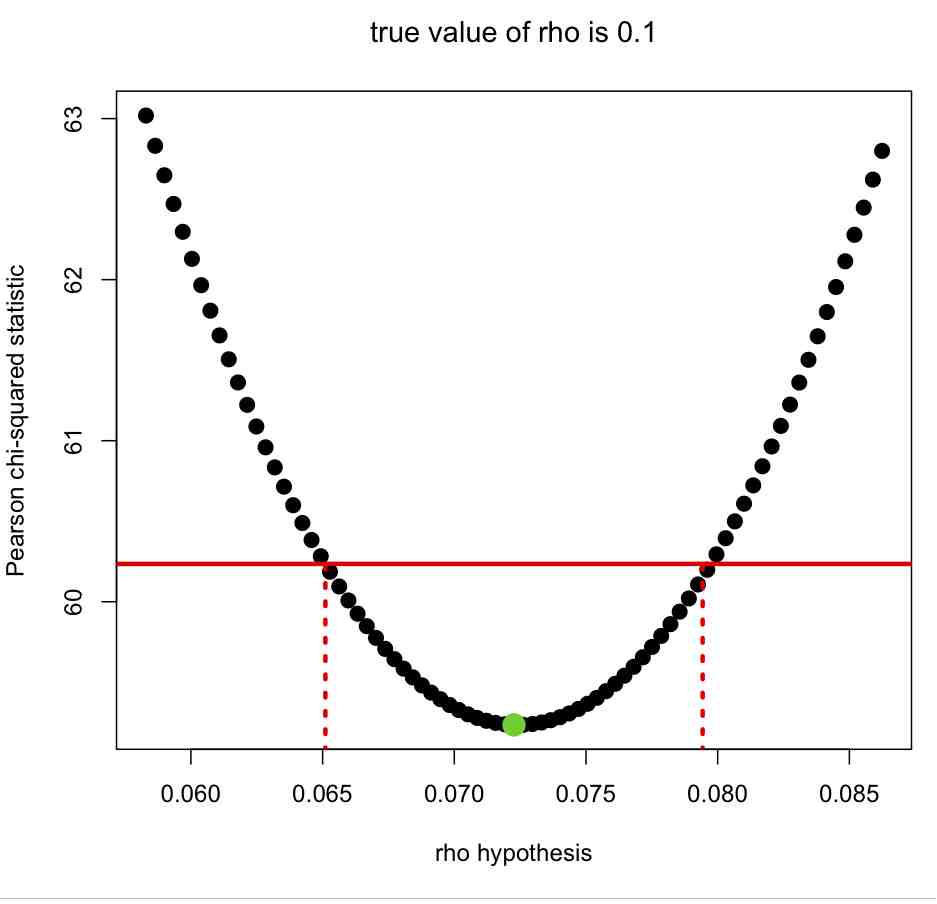
The R script calculates the estimated rho, rho_est, and uncertainty on the estimate, delta_rho_est for each of the 250 simulated data samples that were smeared with the NB distribution, and for each of the 250 simulated data samples that were smeared with the Poisson distribution. It produces this plot, which is the distribution of
n=(rho_est-rho_true)/delta_rho_est
Does the Pearson chi-squared method yields unbiased and efficient estimators for the true rate of exponential rise in our simulated data? Well, for the data smeared with the NB distribution, the script tells us that the mean and standard deviation of n are mu=-1.09 and sigma=2.64. We calculate the uncertainty on mu as delta_mu=sigma/sqrt(N) and get delta_mu = 2.64/sqrt(250)=0.17 We thus test the null hypothesis that mu=0 with S=(mu-0)/delta_mu which yields S=(-1.09-0)/0.17 = 6.42. This gives p-value=1-pchisq(S^2,1)<<0.001. We thus reject the null hypothesis, and conclude that the Pearson chi-squared method produces estimates of the exponential rise that are biased too low when the underlying stochasticity in the data is NB.
We test the null hypothesis that sigma=1 by first calculating delta_sigma=sigma/sqrt(2N)=0.12 and S = (sigma-1)/delta_sigma = 13.7. We thus get p-value = 1 – pchisq(S^2,1) <<0.001. We thus reject the null hypothesis that the Pearson chi-squared method produces efficient estimates of the uncertainty on the exponential rise, and conclude that the uncertainty estimates are biased too low.
Note here that I am so far being very verbose in my description of the hypothesis tests, making it very clear what the null hypotheses were, whether we accepted or rejected them, and what we ultimately concluded. Usually the description is shorter, and doesn’t describe the calculation of delta_mu and delta_sigma (because it is assumed that the reader implicitly knows that they were calculated, and how they were calculated). I give the full description here because I think it is probably useful for people who have never seen how to do this before to understand the full process involved.
Finally, let us examine the performance of the Pearson chi-squared method when using it to fit the exponential rise of data with underlying Poisson stochasticity; the script tells us that from normalized residuals calculated from the 250 trials mu=-0.52, and sigma = 1.08. We thus determine that the p-value testing the hypothesis that mu=0 is p<<0.001. We also determine that the p-value testing the hypothesis that sigma=1 is p=0.91; we thus conclude that the estimates of rho are biased too low, but that the estimates of the uncertainty on rho are efficient.
The Poisson maximum likelihood method
When case counts within each day/week/month bin are low, the method of choice for parameter estimation is the Maximum Likelihood. It has been widely used for decades in fields such as physics. However it is only recently starting to gain traction in computational epidemiology, in part because it is not quite as conceptually easy as LS or Pearson chi-squared for non-statisticians to understand (and nearly all reviewers of any analysis you might publish in computational analysis have very little background in statistical data analysis). However, in the case of fitting to an exponential rise, the use of this somewhat more complicated method is often warranted for the reasons I outlined above.
The ML method maximizes the probability of observing the data, given a model prediction (for instance, the prediction from an exponential curve with some rate, rho) and an assumed probability distribution that underlies the stochasticity within each bin (for instance, the Poisson distribution).
Let’s give an example: an exponential curve with some assumed rate, rho, predicts that the expected average number within a data bin should be lambda=1,000. But the observed number of accounts in that bin is k=3. Let’s assume that the Poisson distribution underlies the stochasticity. Can you see that the probability (ie; likelihood) of observing 3 if the expected average is 1,000 is very, *very* tiny?
How about, if for some other assumption of rho, the exponential curve model predicts that the expected average number in that bin is lambda=4. The likelihood of observing k=3 if the expected average is 4 (with underlying Poisson stochasiticity) is pretty good. The best-fit value of rho is the one that maximizes the likelihood of observing the data!
The Poisson probability (likelihood) of observing k counts when the expected average is lambda is

But in reality, we aren’t just fitting to one bin, we are fitting to a time series with N bins. We thus have to find the rho (the expected number of counts in each bin, lambda, is a function of rho and the time) that maximizes the overall probability of observing those N data points k_i, at times t_i,where i=1,…,N. If the data bins are independent*** of each other, then this amounts to just maximizing the product of probabilities for each bin. In statistics-ese, this means we need to maximize
Which for the Poisson distribution reduces to

Note that whatever rho maximizes the product of probabilities will also maximize the sum of the logarithms of the probabilities. Computationally, a sum of logarithms is much easier to work with than a bunch of produces, and when L is maximized, so is log(L). Thus, the Poisson maximum likelihood method usually involves finding the parameters that maximize
A little bit of algebra gives us
Note that log(k_i!) depends only on the data, not the parameters, thus it is usually just dropped from the likelihood. We thus have the Poisson maximum likelihood is
 (1)
(1)
Just to re-iterate, in case you got lost along the way in this derivation: k_i is the observed number of counts in the i^th time bin (time t_i). The model prediction for the number of counts in that bin is

where the theta is the vector of all the parameters in the model. Note that the model prediction could be an exponential curve (with the rate of rise as the parameter), or it could be an SIR model (with beta as a parameter), or it could be any other model. The form of the likelihood that must be maximized is always that of Equation (1) if you assume that the stochasticity in each data bin is Poisson distributed.
In the maximum likelihood method, traditionally involves minimizing the -log(L). This is probably to make it conceptually similar to a method like least squares.
Estimation of Parameter Confidence Intervals: any Likelihood Method
(not just Poisson)
The covariance matrix for the uncertainty on the parameter estimates, theta, is obtained from the inverse of the Hessian matrix of log(L), calculated at the best-fit value of theta; the Hessian describes the local curvature of a function of many variables, thus large curvature near the minimum indicates that the parameter will have a small uncertainty because log(L) rapidly gets larger as theta departs even a small amount from the best-fit value.

In the large sample limit, the parameter estimates are Normally distributed, so L has a multi-dimensional Gaussian form, and, and log(L) is a hyperparabolic. Thus the s-standard deviation confidence interval can be obtained from the values of theta that satisfy:

Estimation of the rate of exponential rise: Poisson Maximum Likelihood Method
Returning to our special case of fitting to initial epidemic data for the rate of exponential rise: The function for an exponential curve is

Epidemic data are aggregated into bins of a day/week/month, thus the model prediction for a bin that ends at time t_i is
where delta_t is the time span of the bin. This yields
We also have to have the sum of the predicted values equal the sum of the data (this is called “normalizing the likelihood”). This yields
Thus given a value of rho, this constrains alpha to be
The R file fit_exp_with_pois_like.R reads in our simulated data sets, and the uses the Poisson maximum likelihood method to estimate the value of the exponential rise for each of the data sets.
The R script determines the estimated rho, rho_est, and uncertainty on the estimate, delta_rho_est for each of the 250 simulated data samples that were smeared with the NB distribution, and for each of the 250 simulated data samples that were smeared with the Poisson distribution. It produces this plot, which is the distribution of
n=(rho_est-rho_true)/delta_rho_est
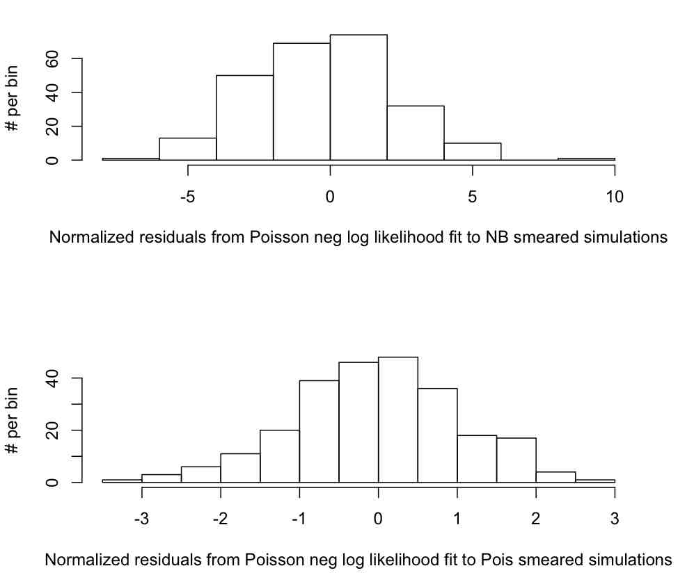
The script also gives the mean and variance of n for the NB smeared data to be mu=-0.25 and sigma = 2.43. The p-values testing the hypotheses that mu=0 and sigma=1, are thus p=0.89 and p<<0.0001, respectively. We thus accept the null hypothesis that the method returns unbiased values of rho, but reject the null hypothesis that the estimates of the uncertainty on rho are efficient (and instead conclude they are biased too low).
The script gives the mean and variance of n for the Poisson smeared data to be mu=-0.03 and sigma = 1.06. The p-values testing the hypotheses that mu=0 and sigma=1, are p=0.35 and p=0.82, respectively. We thus accept the null hypotheses that the rho parameter estimates are unbiased and efficient (YES!)
![]()
Estimation of the rate of exponential rise: Negative Binomial Likelihood
A good reference for the negative binomial likelihood is this paper by Ismail and Jemain. Also, the book Regression Analysis of Count Data, by Cameron and Trivedi. As can be seen in both reference, the Negative Binomial log likelihood isn’t nearly as tidy and compact as the Poisson likelihood, and involves a double sum in the calculation. This can make its use very computationally intensive.
Test for over- or under- dispersion
Most data encountered in epidemiology is over-dispersed due to heterogeneities in the dynamics underlying the spread of the disease. To test for over-dispersion, calculate the statistic

If the data are not over- or under-dispersed, then this statistic should be distributed as chi-squared with N degrees of freedom. For instance, if we have 6 data points, and the data are truly not over- or under-dispersed, in 90% of such cases T will be between 1.6 to 12.6.
This test for dispersion is valid as long as the mean of the Y_i^obs is at least 4 or 5 or so.
Correction for over-dispersion
If the data are appropriate for the application of a Pearson chi-squared fit, a standard method for correction of over- or under-dispersion developed by McCullagh and Nelder is to multiply the Pearson chi-squared statistic, T, by (N-p)/T_best, where T_best is the value of the Pearson chi-squared statistic at the best-fit values of the model parameters, and p is the number of parameters being fit for. We would then determine the uncertainties on the parameters through examination of T’=(N-p)/T_best, rather than T.
If the data are appropriate for the application of Poisson maximum likelihood (ie; low bin counts in many bins), and appear to be over- or under-dispersed via the statistical test described above, then the use of Negative Binomial maximum likelihood method is recommended.
Better method for determination of parameter estimates and their covariance when using the Pearson chi-squared method
As discussed above and also in the previous module, when using the Pearson chi-squared or likelihood method, along with random sampling sweeps of model parameter values, the model parameters can be estimated from the parameter hypothesis for which the figure-of-merit statistic is minimal, and the one standard deviation uncertainty on the parameters is obtained by looking at the range of the parameters that give Pearson chi-squared statistics less than 1 more than the minimum (or negative log likelihood less than 1/2 more than the minimum). We assume that the figure-of-merit statistic has been appropriately scaled if the data are determined to be significantly over- or under-dispersed when compared to the model.
This procedure is only robust if you have many, many sweeps of the model parameter values. It also does not yield a convenient way to determine the covariance between the parameter estimates, without going through the complicated numerical gymnastics of estimating what is known as the Hessian matrix. The Hessian matrix (when maximizing a log likelihood) is a numerical approximation of the matrix of second partial derivatives of the likelihood function, evaluated at the point of the maximum likelihood estimates. Thus, it’s a measure of the steepness of the drop in the likelihood surface as you move away from the best-fit estimate.
There is a much easier way.
If you have many different values of the Pearson chi-squared statistic, T, calculated for different parameter hypotheses, a more robust method for parameter estimation is to calculate the average of the parameter hypotheses, weighted by weights
w=dnorm(sqrt(T-Tmim))
where Tmin is the minimum value of the Pearson chi-squared, and dnorm(x) is the PDF of the Normal distribution evaluated at x (see Section 33.1.2 and 33.1.3 of this reference). The reason that this procedure works better is because it uses information from every single set of parameter hypotheses to obtain an estimate of the best-fit parameter, rather than just the one point at the minimum value of T.
Here is a graphic illustrating the relationship between the distribution of T-min(T) vs the parameter hypothesis for one parameter, and the probability distribution for the parameter: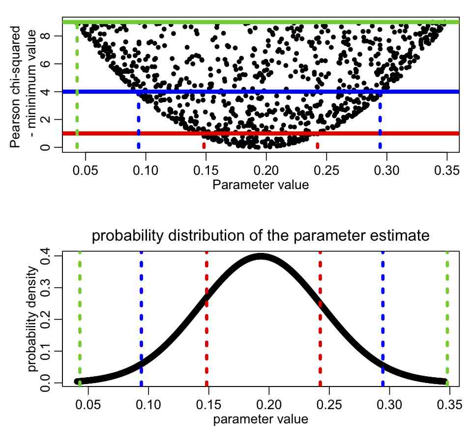
The covariance of the parameter estimates is obtained by calculating the covariance between the parameter hypotheses, weighted by w. There are standard formulas for calculating the weighted mean and covariance. Let’s refer to the i,j^th element of the covariance matrix as V_ij; the one standard deviation uncertainty of the i^th parameter estimate corresponds to sigma_i = sqrt(V_ii). The correlation between the i^th and and j^th parameter estimates is
rho_ij = V_ij/(sigma_i*sigma_j)
Again, the reason that this weighting method provides better estimates of the parameter one standard deviation uncertainties, sigma_i, is because it uses the information from every single set of parameter hypotheses that you have tried, rather than the information from just those that produce a value of T<(min(T)+1).
The R script example_estimation_with_weights.R gives an example of this procedure, fitting the parameters of a parabola y=A*x^2+B*x+C to 100 different data sets that have been randomly smeared using the Poisson distribution. The script produces the following plot. Note that the parameter estimate and one standard deviation uncertainty obtained from the weighting procedure is virtually identical the estimate obtained from examining the range of parameters with T<[min(T)+1]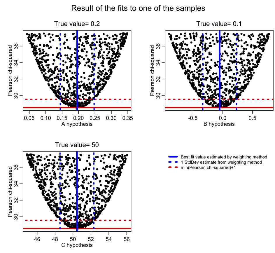
Note that this procedure only works reliably if the parameter values have been uniformly sampled over their range. If the parameters are preferentially sampled from some probability distribution other than the Uniform distribution (for instance, preferentially sampled from a multivariate Normal distribution in order to increase the efficiency of the algorithm), then the weight w has to be divided by the value of the sampling probability distribution at each point sampled.
This weight correction is done in example_estimation_with_weights_b.R (note that the R mvtnorm library needs to be installed in order to use a function that randomly samples from a multivariate Normal distribution). Instead of uniformly sampling hypotheses for the parameters of the parabola, they are preferentially sampled close to the true values from a multivariate Normal distribution.
Try running the script with lcorrect=0 (which will not apply sampling distribution correction to the weights w), and with lcorrect=1 (which will apply the sampling distribution correction). Note that in the former case the estimates of the parameter uncertainties are not efficient, but this problem is corrected in the latter case.
Fitting the parameters of a model to data using parameter sweeps can be done iteratively, where in the first pass the parameters are sampled from the Uniform distribution. Then the Pearson chi-squared or negative log-likelihood statistics calculated in the first sweep are used to determine weights which are used to estimate the parameters and their covariance. In the next step, the parameters are preferentially sampled from a multivariate Normal distribution with these means and the covariance matrix. The process is continued, continually updating the parameters of the multivariate Normal distribution used to randomly sample the parameters. This paper gives a description of an iterative Kalman filter fitting method not dis-similar to the procedure described here. In particular, examine Figure 11.1 in the paper.